This Value at Risk EXCEL example shows how to calculate VaR in EXCEL using two different methods (Variance Covariance and Historical Simulation) with publicly available data.
What you will need
- The Value at Risk resource and reference page.
- Data set for Gold spot prices for the period 1-Jun-2011 to 29-Jun-2012. Download from Onlygold.com.
- Data set for WTI Crude Oil spot prices for the period 1-Jun-2011 to 29-Jun-2012. Download from EIA.gov.
We cover the Variance Covariance (VCV) and Historical Simulation (HS) methods for calculating Value at Risk (VaR).
In the list below the first 6 items pertain to VCV approach while the final 3 items relate to the Historical Simulation approach. Within the VCV approach, we consider two separate methodologies for determining the underlying volatility of returns; Simple Moving Average (SMA) method & the Exponentially weighted moving average (EWMA) method. We do not cover VaR using Monte Carlo Simulation in this post.
We will showcase calculations for in the Value at Risk EXCEL example:
- SMA daily volatility
- SMA daily VaR
- J-day holding SMA VaR
- Portfolio holding SMA VaR
- EWMA daily volatility
- J-day holding period EWMA VaR
- Historical simulation daily VaR
- Historical simulation J-day holding VaR
- 10-day holding historical simulation VaR loss amount for a 99% confidence level
Context
Our portfolio comprises of physical exposure to 100 troy ounces of gold and 1000 barrels of WTI Crude. The price of Gold (per troy ounce) is $1,598.50 and the price of WTI (per barrel) is $85.04 on 29-Jun-2012.
i. Data – Price time series
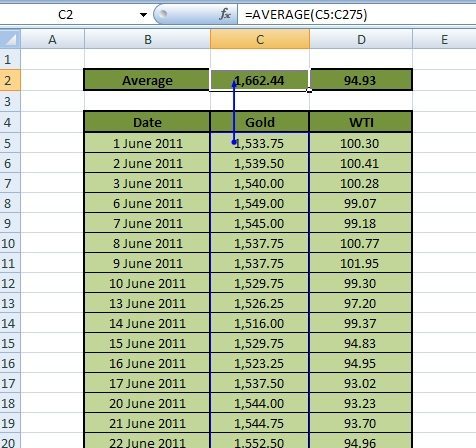
Obtain the historical price data for Gold and WTI for the period 1-Jun-2011 to 29-Jun-2012 from onlygold.com and eia.gov respectively. The period considered in the VaR calculation is the lookback period. It is the time over which we will evaluate the risk. Figure 1 shows an extract of the daily time series data:
ii. Return Series
The first step for any of the VaR approaches is the determination of the return series. We achieve this by taking the natural logarithm of the ratio of successive prices as shown in Figure 2:
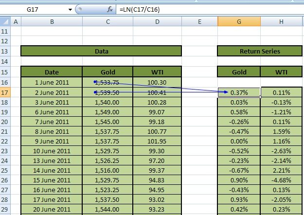
For example, calculate the daily return for Gold on 2-Jun-2011 (Cell G17) as LN(Cell C17/Cell C16) = ln(1539.50/1533.75) = 0.37%.
Variance Covariance – Simple Moving Average (SMA)
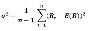
Next, calculate SMA daily volatility. The formula is as follows:
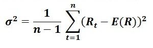
Rt is the rate of return at time t. E(R) is the mean of the return distribution which we can calculate in EXCEL by taking the average of the return series, i.e. AVERAGE (array of return series). Sum the squared differences of Rt over E(R) across all data points and divide the result by the number of returns in the series less one to obtain the variance.
The square root of the result is the standard deviation or SMA volatility of the return series. Alternately, calculate the volatility directly in EXCEL by using STDEV function, applying it to the return series, as in Figure 3 below:
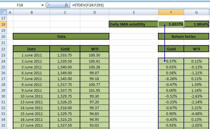
Calculate the daily SMA volatility for Gold in Cell F18 as STDEV(array of Gold return series). The daily SMA volatilities for Gold is 1.4377 % and WTI is 1.9856%.
SMA daily VaR
How much do you stand to lose, over a given holding period and with a given probability? VaR measures the worst case loss likely to be booked on a portfolio over a holding period with a given probability or confidence level.
As an example, assuming a 99% confidence level, a VaR of USD 1 million over a ten day holding period means that there is only a one percent chance that losses will exceed USD 1 over the next ten days.
The SMA and EWMA approaches to VaR assume that the daily returns follow a normal distribution. Calculate the daily VaR for a specified confidence level as:
Daily VaR = Volatility or standard deviation of return series × z- value of the inverse of the standard normal cumulative distribution function (CDF) corresponding with a specified confidence level.
We can now answer the following question:
What is the daily SMA VaR for Gold and WTI at a confidence level of 99%?
Figure 4 shows the calculation below:
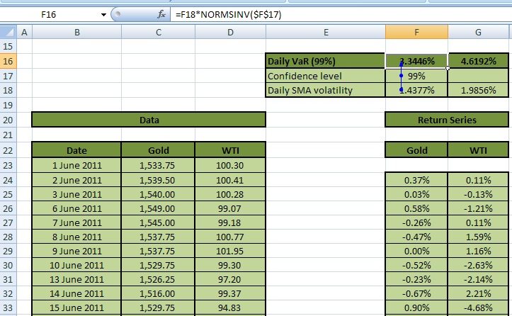
Daily VaR for Gold calculated in Cell F16 is the product of the daily SMA volatility (Cell F18) and the z-value of the inverse of the standard normal CDF for 99%. In EXCEL we calculate the inverse z-score at the 99% confidence level as NORMSINV (99%) = 2.326. Hence, daily VaR for Gold and WTI at the 99% confidence level works out to 3.3446% and 4.6192% respectively.
J-day holding SMA VaR – Scenario 1
The definition of VaR mentioned above considers three things, maximum loss, probability and holding period. The holding period is the time it would take to liquidate the asset/ portfolio in the market. In Basel II and Basel III a ten-day holding period is a standard assumption.
How do you incorporate the holding period into your calculations? What is the holding SMA VaR for WTI & Gold for a holding period 10 days at a confidence level of 99%? Holding period VaR = Daily VaR × SQRT (holding period in days)
Where SQRT(.) is EXCEL’s square root function.
Figure 5 demonstrates this for the WTI and Gold below:
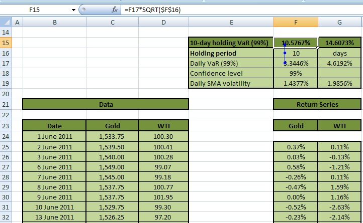
Calculate the 10-day holding VaR for Gold at the 99% confidence level (Cell F15) is by multiplying Daily VaR (Cell F17) with the square root of the holding period (Cell F16). This works out to be 10.5767% for Gold and 14.6073% for WTI.
J-day holding SMA VaR – Scenario 2
Let’s consider the following question:
What is the holding SMA VaR for Gold & WTI for a holding period 252 days at a confidence level of 75%? Note that 252 days represent trading days in a year.
The methodology is the same as used before for calculating the 10-day holding SMA VaR at a 99% confidence level, except that the confidence level and holding period are changed. Hence, we first determine the daily VaR at the 75% confidence level. Recall that the daily VaR is the product of the daily SMA volatility of underlying returns and the inverse z-score (here calculated for 75%, i.e. NORMSINV(75%)= 0.6745). The resulting daily VaR is then multiplied with the square root of 252 days to arrive at the holding VaR.
This is illustrated in Figure 6 below:
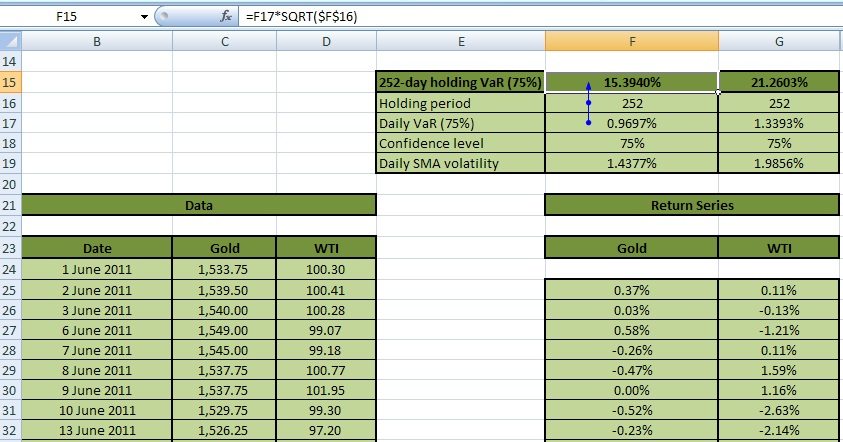
252-day holding VaR at 75% for Gold (Cell F15) is the product of the daily VaR calculated at 75% confidence level (Cell F17) and the square root of the holding period (Cell F16). It is 15.3940% for Gold and 21.2603% for WTI. The daily VaR in turn is the product of the daily SMA volatility (Cell F19) and the inverse z-score associated with the confidence level (Cell F18).
Portfolio holding SMA VaR
We have up to now only considered the calculation of VaR for individual assets. How do we extend the calculation to portfolio VaR? How can we account for correlations between assets in the determination of portfolio VaR? Let us consider the following question:
What is the 10-day holding SMA VaR for a portfolio of Gold and WTI at a confidence level of 99%?
a. Calculation of weights
The first step in this calculation is the determination of weights for Gold and WTI with respect to the portfolio. Let us revisit the portfolio information mentioned at the beginning of the case study:
“The portfolio comprises of 100 troy ounces of gold and 1000 barrels of WTI Crude. The price of Gold (per troy ounce) is $1,598.50 and the price of WTI (per barrel) is $85.04 on 29-Jun-2012.”
Figure 7 shows the calculation of weights below:
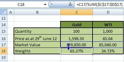
Assess weights based on the market value of the portfolio on 29-Jun-2012. Calculate market values of assets by multiplying the quantity of a given asset in the portfolio with its market price on 29-Jun-2012. Weights are then calculated as the market value of assets divided by the market value of the portfolio where the market value of the portfolio is the sum of market values across all assets in the portfolio.
b. Calculation of Returns
Next, we determined a weighted average return for the portfolio for each data point (date). Figure 8 illustrates this below:
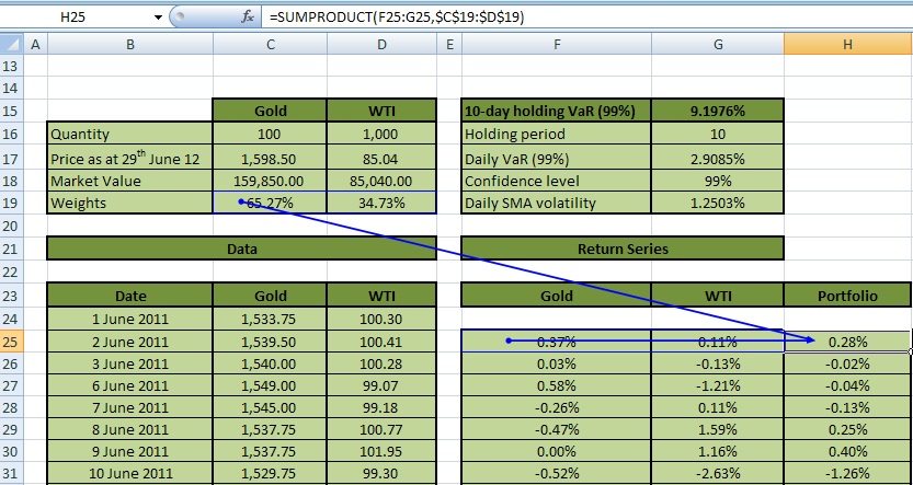
Weighted average return of the portfolio for a particular date is calculated as the sum across all assets of the product of the assets return for that date and the weights. For example for 2-Jun-2011 the portfolio return is calculated as (0.37%*65.27%) + (0.11%*34.73%) =0.28%. This may be done in EXCEL using the SUMPRODUCT function as shown in the function bar of Figure 8 above, applied to the weights row (Cell C19 to Cell D19) and return rows (Cell Fxx to Cell Gxx) for each date. To keep the weight row constant in the formula, when it is copied and pasted over the range of data points, dollar signs are applied to the weights row cell references (i.e. $C$19:$D$19).
c. Portfolio SMA vol & VaR
To calculate the volatility, daily VaR and holding period VaR for the portfolio apply the same formulas as used for the individual assets. That is, daily SMA volatility for the portfolio = STDEV (array of portfolio returns); SMA daily VaR for the portfolio = Daily Volatility * NORMSINV(X); and Holding period VaR for the portfolio = Daily VaR*SQRT (Holding period).
We can now answer the question: What is the 10-day holding SMA VaR for a portfolio of Gold and WTI at a confidence level of 99%? It is 9.1976%.
Variance Covariance Approach – Exponentially weighted moving average (EWMA)
We will now look at how to calculate the exponentially weighted moving average (EWMA) VCV VaR. The difference between the EWMA & SMA methods to the VCV approach lies in the calculation of the underlying volatility of returns. Under SMA, the volatility (σ) is determined (as mentioned earlier) using the following formula:
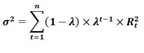
Under EWMA, however, the volatility of the underlying return distribution (σ) is calculated as follows: While the SMA method places equal importance to returns in the series, EWMA places greater emphasis on returns of more recent dates and time periods as information tends to become less relevant over time. This is attained by specifying a parameter lambda (λ), where 0< λ<1, and placing exponentially declining weights on historical data.
The λ value determines the weight-age of the data in the formula so that the smaller the value of λ, the quicker the weight decays. If management expects the volatility to be very unstable then it will give a lot of weight to recent observations while if it expects volatility to be stable that it would give more equal weights to older observations. Figure 9 below shows how we calculate weights used for determining EWMA volatility in EXCEL:
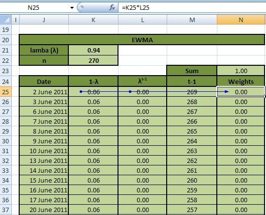
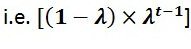
There are 270 returns in our return series. We have used a lambda of 0.94, an industry standard. Let us first look at column M in Figure 9 above. The latest return in the series (for 29-Jun-2012) is assigned t-1=0, return on 28-Jun-2012 will be assigned t-1=1 and so on, so that the first return in our time series 2-Jun-2011 has t-1= 269. The weight is a product of two item 1- lambda (column K) and lambda raised to the power of t-1 (column L). For example, the weight on 2-Jun-2011 (Cell N25) will be Cell K25* Cell L25.
Scaled Weights
As the sum of the weights is not equal to 1 it is necessary to scale them in order that their sum equals unity. This is done by dividing the weights calculated above by 1- λn, where n is the number of returns in the series. Figure 10 shows this below:
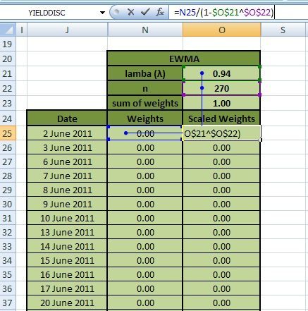
Scaled weight for 2-Jun-2011 (Cell O25) = Weight/(1- λn) = (Cell N25) /(1-Cell O21^Cell O22)
EWMA Variance
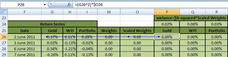
EWMA Variance is simply the sum across all data points of the multiplication of squared returns and the scaled weights. You can see how the product of the squared returns and scaled weights is calculated in the function bar of Figure 11 below:
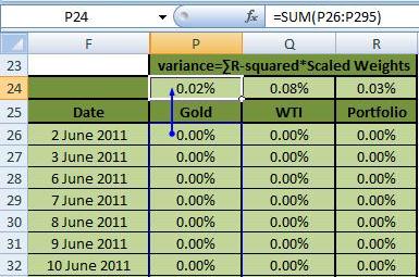
Once you have obtained this product series of weights times squared return series, sum up the entire series to obtain the variance (see Figure 12 below). We calculate this variance for Gold, WTI & the portfolio (using the market value of assets weighted returns determined earlier):
Daily EWMA Volatility
We calculate the daily EWMA volatility for Gold, WTI & the portfolio by taking the square root of the variance. The function bar of Figure 13 below shows this for Gold:
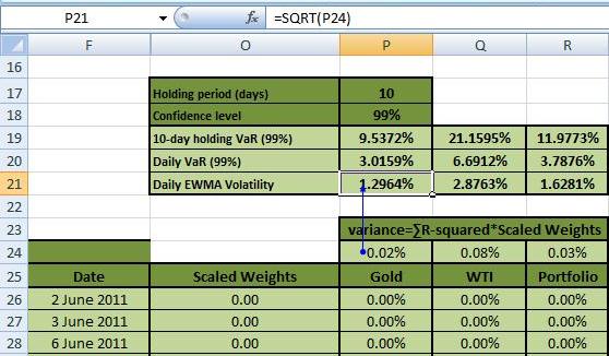
Daily EWMA VaR
Daily EWMA VaR = Daily EWMA volatility * z-value of the inverse standard normal CDF. This is the same process used to determine daily SMA VaR after obtaining daily SMA volatility. Figure 14 shows the calculation of daily EWMA VaR at the 99% confidence level:

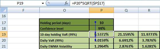
J-Day Holding EWMA VaR
Holding EWMA VaR = Daily EWMA VaR * SQRT(Holding period) which is the same process we use to determine holding SMA VaR after obtaining daily SMA VaR. Figure 15 illustrates the 10-day Holding EWMA VaR below:
Historical Simulation Approach
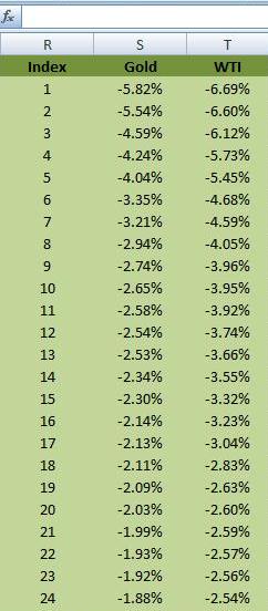
Ordered Returns
Unlike the VCV approach to VaR there is no assumption about the underlying return distribution in the historical simulation approach. VaR is based on the actual return distribution which in turn is based on the data set used in the calculations. The starting point for the calculation of VaR for us then is the return series derived earlier.
Our first order of business is to reorder the series in ascending order, from smallest return to largest return. Assign each ordered return an index value. Figure 16 illustrates this below:
Daily Historical Simulation VaR
There are 270 returns in the series. At the 99% confidence level, the daily VaR under this method equals the return corresponding to the index number calculated as follows:
(1-confidence level)*Number of returns where the result is rounded down to the nearest integer. This integer represents the index number for a given return as shown in Figure 17 below:
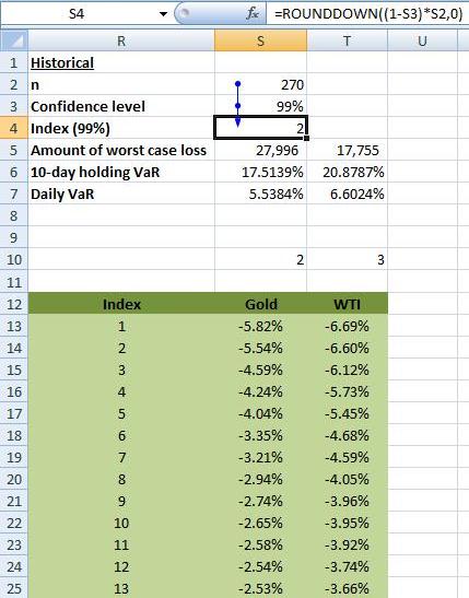
The return corresponding to that index number is the daily historical simulation VaR. Figure 18 shows this below:

The VLOOKUP function lookups the return to the corresponding index value from the order return data set. Note that the formula takes the absolute value of the result. For example, at the 99% confidence level the integer number works out to 2. For Gold this corresponds with the return of -5.5384% or 5.5384% in absolute terms, i.e. there is a 1% chance that the price of Gold will fall by more than 5.5384% over a holding period of 1 day.
10-day holding Historical Simulation VaR
As for the VCV approach, the holding VaR is equal to the daily VaR times the square root of the holding period. For Gold this works out to 5.5384%*SQRT(10) = 17.5139%.
Amount of worst case loss
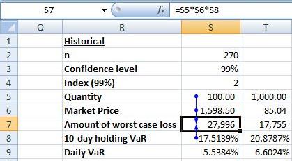
So what is the amount of worst case loss for Gold over a 10-day holding period that will only be exceeded 1 day in 100 days (i.e. 99% confidence level) calculated using the Historical Simulation approach?
Worst Case Loss for Gold @ 99% confidence level over a 10-day holding period = Market Value of Gold * 10-day VaR% = (1598.50*100)* 17.5139%= USD 27,996. There is a 1% chance that the value of Gold in the portfolio will lose an amount greater than USD 27,996 over a holding period of 10-days. Figure 19 summarizes this below:
Comments are closed.