While it is useful to get comfortable with the concept of Delta Hedging, most academic finance specialization programs provide cursory treatment of option price sensitivities and Greeks. Delta hedging as a concept is covered within the foundation of Black Scholes pricing at a theoretical level (single step or two step binomial trees) however actual implementation of a live delta hedging program is something an instructor rarely has time for in the first course on derivative products.

Figure 1 Delta Hedging using Monte Carlo Simulation
Both Mark Broadie and John C Hull have put together illustrative sheets that simulate the actual process of Delta hedging for a call option. This session will help us walk through the basic model and then extend the model in later posts to answer questions around profitability and model behavior.

Figure 2 Delta Hedging – Tracking Error between Replicating portfolio and options
We will also track the error in the model and discuss its sources. The error arises because the replicating portfolio doesn’t track the actual option value perfectly. There is a mismatch and the tracking error shows that.
Monte Carlo Simulation – Delta Hedging Model – Setting the ground
I saw the original model in Mark’s Security Pricing class at Columbia Business School in fall of 1999. Since then the essential model has remained unchanged. We will extend Mark’s model a bit when we evaluate profitability for the option book. The Hull approach is similar to the Broadie method and if you are comfortable with either of the two you will be fine.
For back ground information on Greeks, see the Option Greeks Quick Reference Guide as well as the Derivatives Greeks Interview Guide. Both posts include a review of calculating Delta, Gamma, Vega, Theta & Rho as well as some discussion on the behavior of Delta as you move around Spot, Strike, Interest Rates, Volatility and time to expiry.

Figure 3 Delta Hedging – The baseline model and simulated values
The primary model simulates:
a) The underlying stock price using the Black Scholes equation
b) Option Delta using the simulated underlying price
c) Replicating portfolio comprised of a long position in Delta x S (Spot price of underlying stock) and a short position in Borrowing B.
d) Difference between the replicating portfolio and the option value.
If you are unfamiliar with the basics of Monte Carlo Simulation please see the Monte Caro Simulation Training Guide below as well as our complete collection of posts on Monte Carlo simulation before proceeding further.
For the purpose of our simulation we will start off with Barclays Bank (I know, I know) and assume that the bank will pay no dividends over the life of the option.
Delta Hedging Model using Monte Carlo Simulations – Assumptions
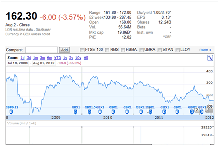
Figure 4 Delta Hedging – Barclays bank price chart
We will assume that the spot price is 162.3, the daily volatility will range between 2.5% to 5%. Implied annualized volatility will be assumed to be 40%. Risk free rate of interest will be 1%, time to maturity will be one year. As discussed above, the stock will pay no dividends.
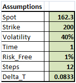
Figure 5 Delta Hedging – Key Assumptions
Using the above assumptions we go ahead and simulate a path of Barclays share price over the next one year using a single month interval. We are assuming that the recurring rebalancing period before the option delta is evaluated and the replicating portfolio is rebalanced is 1 month. The approach will give us 12 prices at monthly intervals, and 12 rebalancing points.
Delta Hedging Model – Monte Carlo – Simulating the stock price
Using our old friend the discrete edition of the Black Scholes equation we go ahead and simulate Barclays share price for the next 12 months.
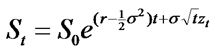
Figure 6 Simulating equity prices
The result should look as under. However our numbers will not match since the random seed used by the Excel RAND() function are going to be different for everyone.
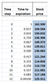
Figure 7 Delta Hedging – Simulated price series
While the first eleven time steps are equidistant, the 12th one is a little short. We have done this by design because we want to examine the option the day before it expires, hence the value .001 rather than 0.
The actual stock price simulation with the original discrete formula and the Excel implementation is shown below.
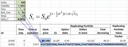
Figure 8 Delta Hedging – Monte Carlo simulation – Excel implementation
Delta Hedging Model – Calculating Delta for our Simulation model
The next step is to calculate d1, d2 and delta values based on the simulated stock prices at each step.
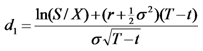
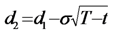
,
The value of d1 and d2 are given by the standard Black Scholes implementation. Option Delta is simply N(d1) or NORMSDIST(d1).
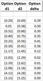
Figure 9 Monte Carlo simulation – d1, d2 & Option delta
Monte Carlo Delta Hedging Model – Calculating Total Borrowing
Now that we have option delta for each simulated stock price at each time step, it takes a simple multiplication step to calculate Dollars in stock (Delta x S).
However total borrowing requires a more involved calculation. At time zero when the option is written total borrowing is given as the difference between Dollars in Stock and the premium received for the option. This is given in the first cell at time zero. It is the second cell at time one where the calculation gets a little messy.
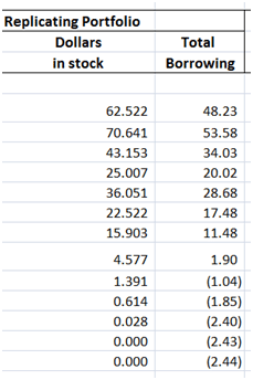
Figure 10 Delta Hedging – Replicating portfolio components
One way of dissecting this calculation is to take a quick and close look at the top four rows of our delta hedge table and just do a simple step by step calculation that shows us how the total borrowing figure changes from one rebalancing period to the next. Its an essential step without which you cannot decode the delta hedging sheet.
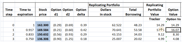
Figure 11 Delta hedging – dissecting total borrowing
At time zero the underlying stock is trading at $162.3. Option delta is 0.39.
We end up buying $62.522 (39% of 1 share) of stock for the hedge.
The purchase is funded by $14.29 in option premium and $48.23 in borrowing. How does this balance change at time step 1?
At time step 1, the underlying stock has moved to 169.584. Our 39% of 1 share is now worth $169.584/162.3 x 62.522 which translates into $65 dollars and change.
In addition option delta has moved from .39 to .42 so we need to buy an incremental 3% of the underlying share at the new price which is another $5 dollars and change. The combined position after the new purchase is 70.641.
So what is the incremental amount that was borrowed to finance the hedge? $5 dollars and change. How did we find the exact number? If you look above and review the calculation again, it’s the difference between the new delta and the old delta multiplied by the new stock price. That is the new net incremental borrowing. When delta and underlying prices fall, the formula will release funds. When they rise it will require funds.
But there is one more step before the total borrowing calculation is complete. What about the previous balance? Balance that was borrowed at step zero. We owe accrued interest on it for one period at the one period (time step) rate. So the actual calculation of total borrowing has two parts – the previous balance + accrued interest and the new borrowing reflecting the change in option delta.
When you put all of this together you end up with the formula used for calculating total borrowing balance at time step 1 in the delta hedge sheet. The same process is used to calculate the total borrowing balance at step 2, step 3 and onwards.
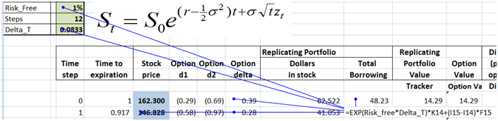
Figure 12 Delta hedging – Marginal borrowing at each time step
Monte Carlo Simulation – Delta Hedge Model – Putting it all together
Replicating portfolio is simply $ in stock (column 7) less Total borrowing (column 8). You can clearly see now that while the replicating portfolio is doing a reasonable job of tracking the option value, there is a clear error in tracking, which moves up and down depending on how much in or out of money the option is.
Figure 13 Delta hedging – the final picture
To calculate option value we use the standard Black Scholes formula for a non-dividend paying stock.
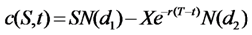
The Excel implementation is shared below.
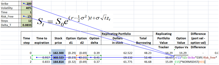
Figure 14 Delta hedging – Option value – excel implementation
Monte Carlo Simulation – Delta Hedging Model – Next questions, steps & homework.
Now that the underlying simulation model is ready for delta hedging, here is a list of questions that we would like to answer.
a) How would this hedging model change if the option contract was a put contract? If our call is hedged by Delta x S – B, what would be required to hedge a put?
b) How do you calculate the P&L for this book? Do you actually end up making money in this business? What are the sources of income and expense?
c) How does implied volatility impact profitability? How is that factored here?
d) To calculate profitability you need the dollar cost average price of purchase for the share? How is that calculated?
e) Once you have a P&L model can you test how profitability behaves as you shorten the rebalancing period? How do other drivers impact profitability?
f) How do the other Greeks behave? Can we also hedge them using a similar approach?
Build the model & think about answering these questions by yourself. We will try and answer some of them in our posts later this month.
To answer these questions you may find it useful to check the Derivatives pricing Greeks Quick Reference Guide, Delta Hedging Cash PnL Simulation as well as the Derivatives Greeks Sales & Trading Interview Guide.
Comments are closed.