Our alternate EXCEL TARF Pricing model uses the Black Scholes close form solution to find a price.
The TARF contract described in the product term sheet above is equal to having a series of forward contracts that buy JPY and sell USD at the Strike rate and a series of short put option positions on Yen. For the options, the client is in effect the writer of the put and is obligated to buy JPY if the option is exercised. The buyer will exercise the option when the JPY depreciates against the USD in relation to the strike. The Notional on both instruments is JPY 200 million.
We will price each of these instruments separately and then add their results together to arrive at the value of the TARF.
Value of Forwards
The value of the forward for each leg can be determined using following formula:
(K-F0) x EXP(-rdt) x USD Notional @ K
Where K is the Strike Rate
F0 = implied forward rate = S0 x EXP((rd-rf)x t)
USD Notional = JPY Notional/K
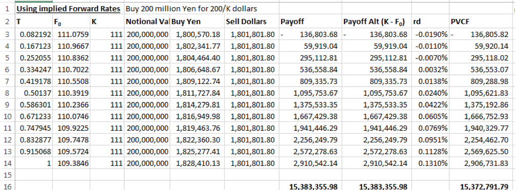
The value of the contract is the sum of the value of each legs forward contract.
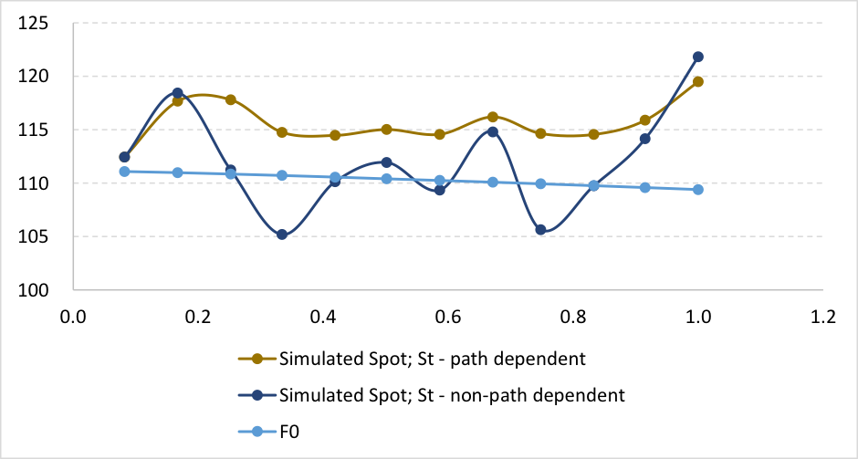
However, as we are comparing the results of the first principles approach with the second combination of derivative instruments approach, we will need to use the simulated spots to determine the values of the forward contracts. We will use the result from the deterministic approach later to assess the accuracy of the results from the simulation model.
In the case of the simulated model, we replace F0, the implied forward rate with the simulated spot rate at the time of expiry. The value of each forward leg will then be:
(K-ST) x EXP (-rd x t) x USD Notional @ K
And the value of the contract will be the sum of values of each leg.
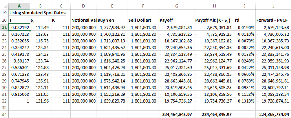
In the screen shot above, Column E = JPY Notional Value /ST
Column F = JPY Notional Value/ K
And the payoff at Column G = Column E – Column F. Alternatively, the value may be arrived at as ( Column C – Column B) * Column F
The present value of payoff for each leg calculated in Column J is Column G x EXP (-Column I x Column A)
The value of the forward contract is the sum of present values across the twelve legs.
The graph below plots discounted payoffs against the ordered simulated spot path.
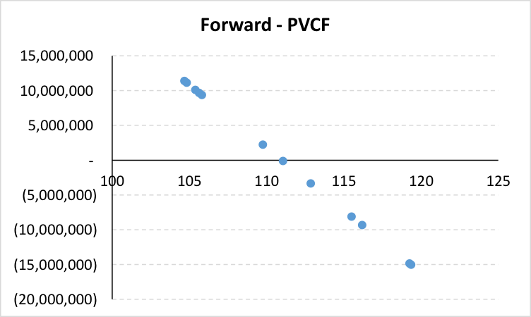
Unlike the TARF payoff graph, the losses are not leveraged when the Japanese Yen depreciates against the US Dollar in relation to the strike.
Value of Put Options
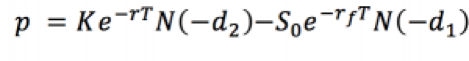
The value of a put option on Japanese Yen is given by the Black Scholes (BS) formula:
As the currency convention mentioned in the term sheet is USD-JPY, the inputs in the formula will be:
S0 = 1/111.17 (inverted initial spot)
K = 1/111 (inverted strike rate)
rd = USD LIBOR
rf = JPY LIBOR
The result for p will be expressed in USD terms. To calculate the total premium and convert to JPY terms, we have:
p x JPY Notional x USD-JPY spot rate at expiry.
To further understand the USD-JPY convention in terms of its application in the BS option pricing formula please click here.
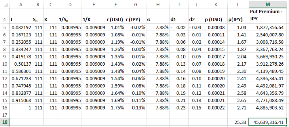
Column K is the calculation of put premium for 1 option contract using the put option formula mentioned above expressed in USD Terms.
Column M gives the total put premium per leg in JPY terms. This is equal to present value of payoffs for a put option buyer. To arrive at the value for the option writer we multiply the result with -1.
As in the case for forwards above, this method gives us a deterministic closed form solution to the value of the series of put options. However, as the first principles approach to calculating the value of the TARF contract is based on simulated spots, we need to recalculate the option value using a simulation model. We will use the result from the deterministic approach later to assess the accuracy of the results from the simulation model.
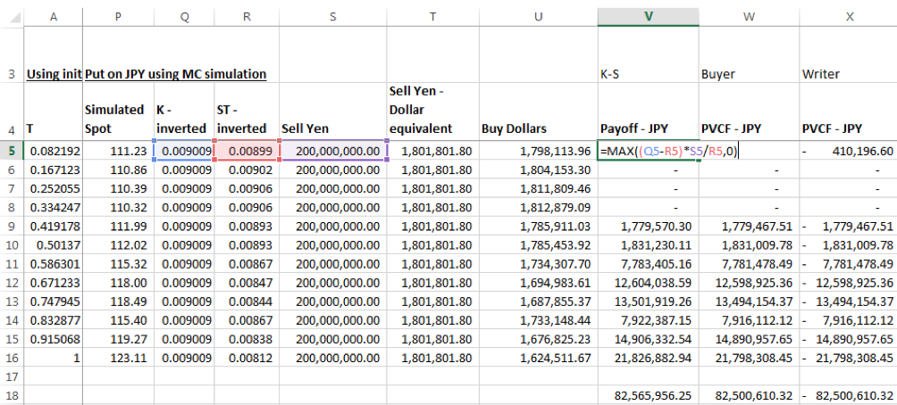
Given the currency convention the Payoff in USD is maximum of (Inverted Strike – Inverted initial Spot, 0) x JPY Notional. To convert to JPY terms this result is multiplied by the USD-JPY spot rate at expiry (alternatively divided by the corresponding JPY-USD rate). The calculation is given in Column V. The discounted value of payoff is given as Payoff (in JPY terms) x discount factor. Discount factor = EXP (-rd x t), where rd is the JPY LIBOR rate.
This present value is the discount value for the buyer of the option. The present value for the seller is equal to -1 times this amount.
The sum of present values across all twelve legs equals the value of the put option.
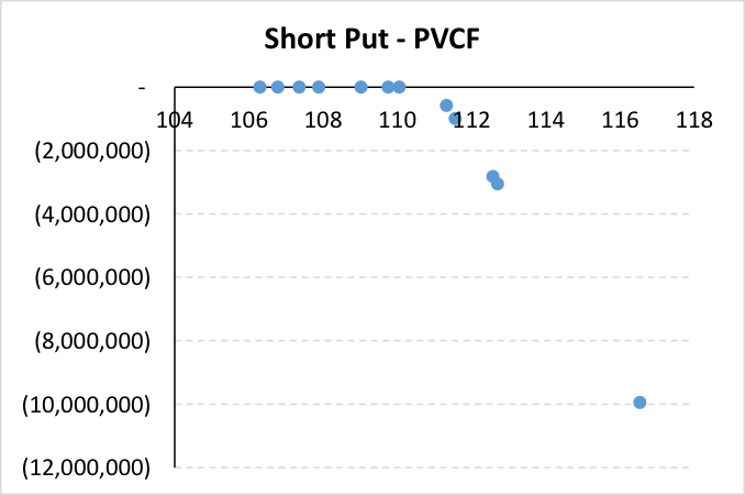
The discounted payoff profile for the series of put options across the legs for one simulation run is depicted below:
TARF – Forward + Short Put
The value of the TARF for each leg will equal the sum of the discounted value of payoff of the forward (long Yen short USD) plus the discounted value of the payoff of the put option for the option writer.
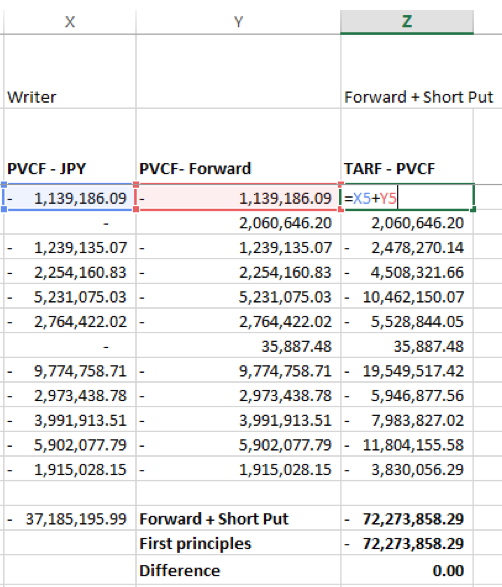
The results from the first principles approach and the sum of derivatives approach match.
Excel TARF Pricing Models – Black Scholes vs Simulation
To evaluate the results from the deterministic and simulation approaches we first generate and store results for 1000 simulated runs from our MC simulation models.
One scenario of average results across 1000 simulated runs is mentioned below. The results are shown against the results from the closed form formulas for forward & option contracts.
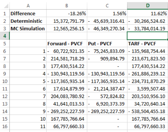
The TARF value is the sum of the Forward and Put contracts results. There is a variance in results between approaches primarily because of the difference in forward contract values. We have observed that the difference tends to be larger in general when the MC simulation models use path-dependent simulated spots than when the simulated spots are non-path dependent. Is there anything we can do to improve the convergence. Turns out the answer is yes and we explore it in our next post.