Our two part series on TARF pricing models begins where we stopped with our analysis on TARF hedge effectiveness. We cover both vanilla TARF (without any path dependent options) and Knock in Knock out (KIKO) TARF’s in that discussion. In this post we start with reviewing our simulation based TARF pricing model.
Definition & Scope
A Target Redemption Forward (TARF) transaction allows a customer to exchange one currency for another at a contract rate that is more attractive compared to the rate on a traditional forward contract. The higher rate is accompanied with a higher level of downside currency exchange risk if the exchange rate were to move in the wrong direction from that expected. The TARF structure is usually comprised of a series of individual legs that redeem on consecutive expiry dates.
This post is a step by step guide to building a TARF model in EXCEL. We address the model building exercise in two ways:
- A first principles approach using the expiry profile mentioned in the term sheet below
- A combination of pricing and summing together the results of conventional derivative products (forwards & options) approach
No-arbitrage pricing in a rational world, means that the results from the two approaches should be the same.
In both models, we make use of a Monte Carlo simulation model to simulate the path of the future spot exchange rates. To check the validity and accuracy of results obtained from the MC simulation we use closed form formulae in the derivatives combo approach mentioned above and compare the average results across 1000 simulation runs with the results arrived at using the deterministic method.
TARF Product term sheet
Let’s begin with defining the term sheet for the plain vanilla TARF that we will be building the pricing models for. The TARF is plain vanilla in that it does not contain any knock in or knock out triggers that would normally be included with such contracts.
| Start date | 31-May-2017 |
| Notional per expiry | JPY 200 Million/ JPY 400 Million |
| Currency Convention | X JPY per 1 USD [USD-JPY] |
| Spot Reference at inception, S0 | 111.17 |
| Strike Rate* | 111 |
| Expiry Profile | If the USD-JPY rate at expiry is greater than the Strike Rate on the expiry date, the client will buy JPY 400 Million versus USD at the strike rate on the settlement date**
If the USD-JPY rate at expiry is less than or equal to the Strike Rate on the expiry date, the client will buy JPY 200 Million versus USD at the strike rate on the settlement date |
| Expiry dates | 30-June-2017
31-July-2017 31-August-2017 30-September-2017 31-October-2017 30-November-2017 31-December-2017 31-January-2018 28-February-2018 31-March-2018 30-April-2018 31-May-2018 |
| Day count convention | Actual/ 365 |
*We have used a constant Strike for all the TARF redemption legs here. This may be easily adjusted so that each leg is subject to a separate strike. The reason for choosing the same strike is to be able to illustrate graphically the payoff profile for the underlying instruments which would not be possible for a varying strike.
**Let us assume for now that the terms expiry dates, settlement dates and delivery dates are equal to each other and used interchangeable. Generally, there would be a lag, typically two days between the expiry date and the settlement/ delivery date.
Model Pricing Data
In order to price the model we require the following data:
- Risk free rates for JPY & USD: We use proxies of JPY LIBOR and the USD LIBOR for these rates. Monthly average rates for the month of May 2017 was obtained from the global-rates.com website. The rates were available for the 1-,2-3-,6- & 12-month tenors. The rates for interim months, 4,5,7,8,9,10 &11 linearly interpolated from these rates.
- Volatility of the USD-JPY exchange rates: Implied volatilities may be obtained from the website investing.com/currencies/usd-jpy-options for various option tenors. For simplicity, we have assumed a constant volatility of 7.88% across all tenors in our pricing models. This may be easily adjusted by using a different volatility for each TARF expiry leg based on the tenor of that leg.
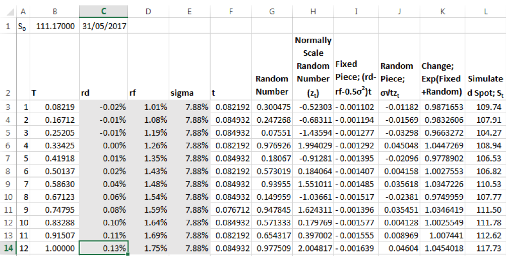
- Simulated future spot USD-JPY rates: To build the MC simulator we use the model described here, with mu replaced by rd-rf, the differential between the domestic risk free rate and the foreign risk free rate. Given that the currency convention is X JPY per 1 USD, the domestic risk free rate is taken as the JPY LIBOR and the foreign risk free rate is taken as the USD LIBOR.
TARF Pricing Model # 1 – First Principles
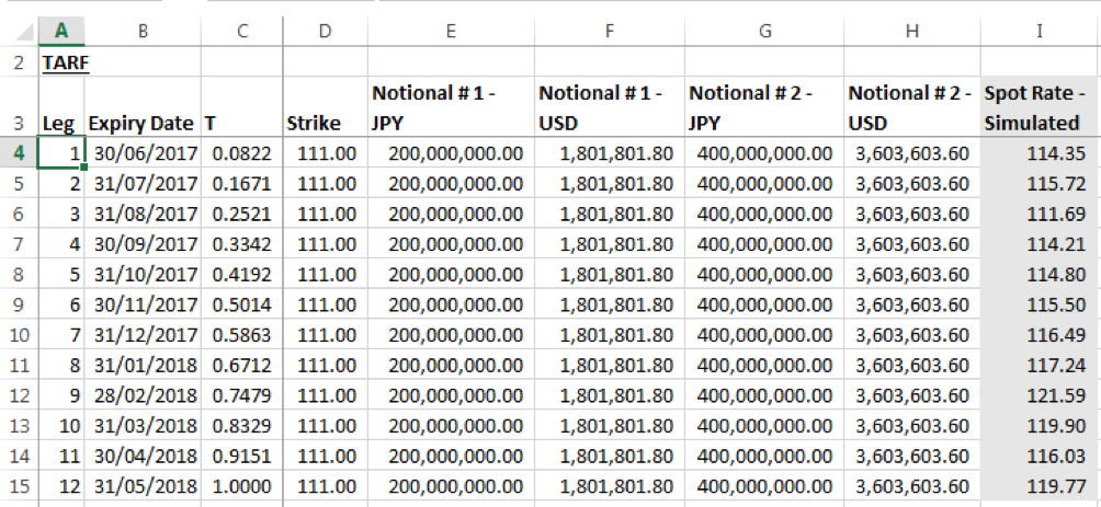
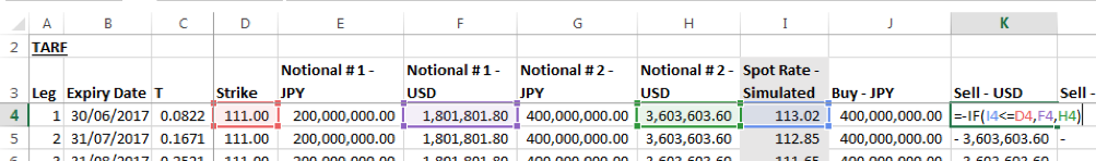
The first part of the model simply lists the details of the term sheet by leg. For example, row 4 show the details of the first leg. The leg will expire on 30-June-2017. This is 30/365 years from the date of inception, our calculation date. The applicable strike is 111. The Notional amounts in JPY are 200 million and 400 million respectively (columns E & G) and the equivalent amounts in USD, given the strike, are simply the JPY notional amounts divided by the strike rate (columns F & H). The simulated spot rate from our MC simulator is called in column I. This is repeated for each of the 12 legs mentioned in the term sheet.
Columns J-P present the working of the payoffs for each leg:
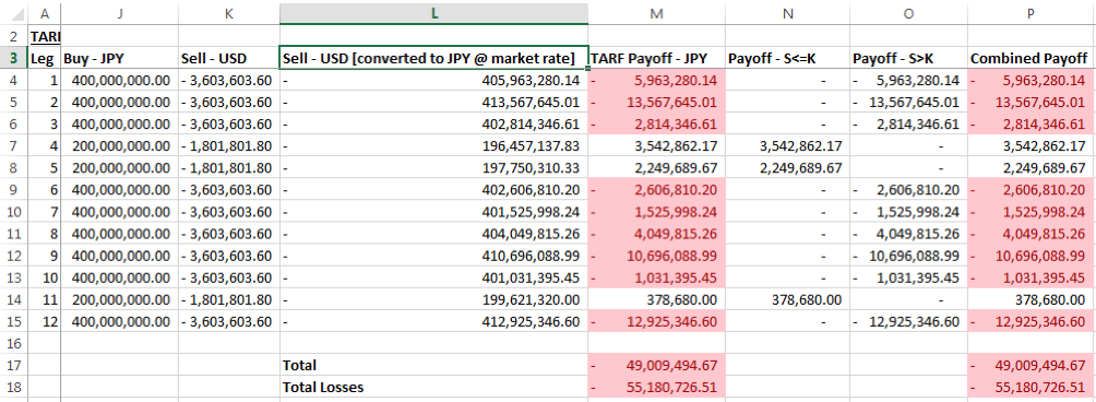
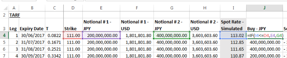
Column J gives the JPY amount that will need to be purchased by the client based on the expiry profile given in the term sheet. The formula in column J includes the condition that if the Simulated Spot Rate at time T is less than or equal to the Strike the Notional used will be JPY 200 million, otherwise, it will be JPY 400 million.
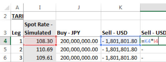
The formula in Column K includes a similar condition for the corresponding USD Notional calculated from the JPY Notional at strike. We have multiplied the result with a -1 to represent the short position in USD.
Column L expresses the value of the USD Notional given in column K in JPY terms (USD notional times the simulated spot rate at time T).
The sum of columns J and L is equal to the TARF Payoff expressed in JPY terms.
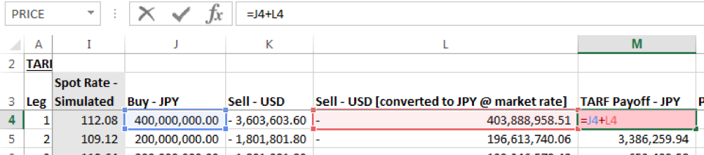
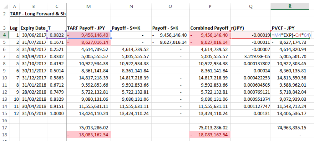
Columns N-P break down this calculation in an alternative manner, with column N showing the payoff when ST<=K only and column O showing the payoff when ST>K only, otherwise a value of zero is returned. The combined payoff at column O, the sum of columns N & P, is equal to the TARF Payoff in column M.
The Price of the TARF is the sum of the present values of cash flow of each leg, where the present value is the payoff discounted over the tenor to the inception date/ date of calculation using the domestic risk free rate, i.e. Payoff x EXP(-rdt). As the payoff is in JPY the domestic risk free rate is the JPY LIBOR.
The graph below documents PV of Payoffs across the legs under one simulated scenario. The graph plots discounted payoffs against the ordered simulated spot path. A clear kink is visible at the strike rate which shows that for a given % change in spot prices in relation to the strike, the losses suffered are higher that the gains made. Note this is a typical outcome that arises from the gearing structure built into a TARF product.
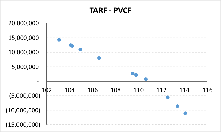

xProduct()