There are three primary methods used for calculating Value at Risk (VaR).
a. The Variance /Covariance method
b. The Historical simulation method
c. The Monte Carlo simulation method
All VaR methods have a common base but diverge in how they actually calculate Value at Risk (VaR). They also have a common problem in assuming that the future will follow the past. Supplement any VAR figures with appropriate sensitivity analysis and/or stress testing to address this shortcoming.
In general, the VAR calculation follows five steps:
- Identification of portfolio positions for calculation of Value at Risk
- Identification of risk factors affecting the valuation of positions.
- Assignment of probabilities (or statistical distribution) to possible risk factors values.
- Creation of pricing functions for positions as a function of values of risk factors.
- Calculation of Value at Risk (VaR)
Variance Covariance method
This VaR method assumes that the daily price returns for a given position follow a normal distribution. From the distribution of daily returns calculated from daily price series, we estimate the standard deviation. The daily Value at Risk VaR is simply a function of the standard deviation and the desired confidence level. In the Variance-Covariance VaR method, calculate the underlying volatility either using a simple moving average (SMA) or an exponentially weighted moving average (EWMA).
Mathematically, the difference lies in the method used to calculate the standard deviation.
This approach is utilized with the assumption that the daily returns during the lookback period follow a normal distribution. We know that this assumption is not true. Especially under times of stress and extreme conditions. But we qualify our presentation by including the assumption and the challenges to its validity in our disclosures.
The SMA approach places equal importance on all returns in the series. The EWMA approach places greater emphasis on returns of a more recent duration.
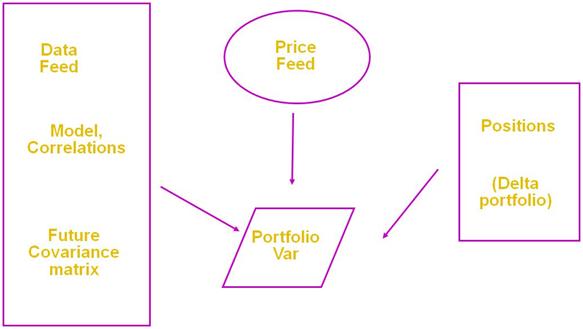
The Variance-Covariance VaR method makes a number of assumptions. The accuracy of the results depends on how valid these assumptions are. The method gets its name from the variance-covariance matrix of positions that it uses as an intermediate step to calculate Value at Risk (VaR).
The method starts by calculating the standard deviation and correlation. It then uses these values to calculate the standard deviations and correlation for the changes in the value of the individual securities that contribute to the position. If price, variance and correlation data is available for individual securities then use this information directly. Then use the values to calculate the standard deviation of the portfolio by matrix multiplication.
Calculate Value at Risk (VaR) for a specific confidence interval by multiplying the standard deviation by the appropriate normal distribution factor.
A modified approach to VCV VaR
In some cases, a method equivalent to the variance covariance approach is used to calculate VAR. This method does not generate the variance covariance matrix and uses the following approach:
- Separate the portfolio in a long side and a short side.
- Calculate the return series for the long side and the short side.
- Use the return series to calculate the correlation and variances for the long and short sides
- Use the results in (3) to calculate the VaR.
The modified approach can be used where, due to the nature of the institutional strategy, a number of positions would net close to zero on a portfolio basis. Also, where the set of securities employed is so large that a variance covariance approach would have significant resource/time requirements.
Historical Simulation Method for Value at Risk (VaR)
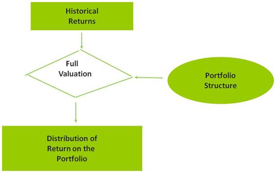
This approach requires fewer statistical assumptions for underlying market factors. It applies the historical (100 days) changes in price levels to current market prices to generate a hypothetical data set. Then order the data set is by the size of gains/losses. Value at Risk (VaR) is the value that is equaled or exceeded the required percentage of times (1, 5, 10).
Historical simulation is a non-parametric approach of estimating VaR, i.e. the returns are not subjected to any functional distribution. Estimate VaR directly from the data without deriving parameters or making assumptions about the entire distribution of the data. This methodology is based on the premise that the pattern of historical returns is indicative of future returns.
Monte Carlo Simulation for calculating Value at Risk (VaR)
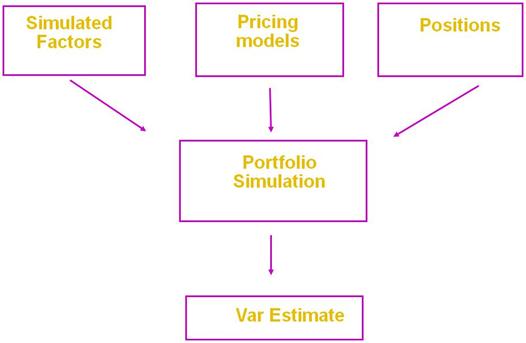
The approach is similar to the Historical simulation method described above except for one big difference. The hypothetical data set used is generated by a statistical distribution rather than historical price levels. The assumption is that the selected distribution captures or reasonably approximates price behavior of the modeled securities.
A Monte Carlo simulator uses random numbers to simulate the real world. A Monte Carlo VaR model using the following sequence of steps
- Generate randomly simulated prices
- Calculate daily return series
- Repeat the steps in the historical simulation method described below
Quick Review
| Historical Simulation VaR | Variance / Covariance VaR | Monte Carlo Simulation VaR | |
| Risks of portfolios that contain options | Yes regardless of the option content | No, except when computed using a short holding period with limited or moderate option content | Yes, regardless of the option content |
| VaR Computation performed quickly | Yes | Yes | No, except for relatively small portfolios |
| VaR method easy to explain to senior management | Yes | No | No |
| Misleading VAR estimates when recent past is not representative | Yes | Yes, except that alternative correlation may be used | Yes, except that alternative correlation may be used |
| Scenario analysis | No | Easy to examine assumptions about variances and correlation. Unable to examine alternative assumptions about the distribution of market factors | Yes |
Implementing Value at Risk (VaR)
The objective of a Value at Risk (VaR) implementation is to perform daily VaR analysis of positions within a portfolio. Such a process would be the first step in shifting the current emphasis from calculating VaR to managing VaR. Within the process the focus should be on:
- Positions with low coverage levels.
- Portfolio positions with VaR beyond a set threshold.
- Positions with significant VaR changes.
- VaR analysis for the Desk. (All clients, All accounts, All positions)
Value at risk – implementation challenges and recommendations
From a methodology point of view, the most robust results are likely to come from the historical simulation approach. This happens because the approach is not handicapped by the normal distribution assumption. The VCV approach is the most popular approach. However, it is also the one that receives the most criticism given the normality assumption.
The Monte Carlo approach appears to be fairly attractive but in most simulators, the default distribution used is also normal. This essentially puts the results in the same category and range as the VCV approach. The big benefit of the simulation approach is when actual trade price data is not available and prices and returns need to be derived for market factors. This happens especially when portfolio positions include exotic OTC derivative contracts.
There are a number of tweaks and hacks for building simulators that use the true distribution rather than a simulated normal distribution.
Comments are closed.