My love affair with Monte Carlo Simulation
Let’s start with the honest truth. I had a torrid long distance love affair with Monte Carlo simulation over many years that ended up badly in a painful breakup.
This is not going to be a neutral post. To say that I will be biased is an understatement. But to be fair here is the concise version of our love story.

In 2004 we wrote the risk management engine for a derivatives portfolio. The client was a large emerging market bank. The portfolio included FX options, FX participating forwards, long dated Interest Rate Swaps and Cross Currency Swaps.
It wasn’t supposed to be a big deal till we started factoring emerging market drivers, absence of secondary market trades, public quote data, trading volumes, market crises, crashes and biases. We had been working with Monte Carlo simulations for the last four years and for someone deeply, madly in love with the algorithm, the simulation model was a natural choice.
Since this was a risk platform the objective was to forecast a Value at Risk (VaR) number that the bank could use for internal capital allocation. None of the positions traded publicly, however data on the underlying currencies and rates was publicly available and quoted. The simulation model would simulate the underlying rates, mark to market the portfolio using the simulated rates, calculate the daily simulated price change and repeat the simulation exercise for the next 12 months. We would pick through the wreckage of simulated crises and crashes and identify the Value at Risk estimate.
The implementation was elegant, a bit complex but an overall success till the traders on the market making desk saw the results and threw them in a trash bin. I was heartbroken and disappointed but I knew in my heart that the traders were right. We had looked at the results and despite our calibration and tweaks knew that we were under estimating the true exposure. We lost the client, killed the model and moved on to other alternate solutions.
Monte Carlo Simulation revisited – Fixing the distribution
Over the years we played with many different alternates but I always wanted to fix that hole that my original love affair with Monte Carlo had left. I became a big fan of the Historical Simulation model for calculating Value at Risk but wondered what would happen if I could bring the two approaches together. Run a simulation using the Monte Carlo method, but use the true distribution rather than the default Normal selection simulation models pick.
In 2009, working on another simulation exercise we did exactly that. This time the portfolio was collection of cross currency swaps. The question once again was capital allocation for the position, the issue was estimating Value at Risk (VaR). We picked up historical rates, ran a simulation using historical rates and returns, marked to market the portfolio using simulated historical returns.
The original Monte Carlo Simulation model use the following process:

The revised hybrid approach tweaked it to the following variant.

The results were very interesting. Much more real, and certainly a lot more acceptable to the traders. The approach made sense specifically for valuing exotic, illiquid, non-traded securities and positions that were dependent on traded, quoted underlying securities, currencies, rates or commodities. It was even more useful for emerging market exposure where simple simulation models would break down because they couldn’t factor in the volatility of the underlying emerging market variables.
The Hybrid Monte Carlo Simulation Model – Using the actual historical distribution
Last week while working through some down time we re-ran our models for three interesting commodities and one currency.
- Oil – Spot prices – WTI Bench Mark
- Gold
- Silver
- Euro-USD Exchange rate
The remaining part of this post presents the results of our analysis.
Monte Carlo simulation and historical returns – Calculating Value at Risk (VaR)
A natural question that should come up after the above discussion is how does the hybrid Monte Carlo simulation model using historical returns fare in terms of Value at Risk measurement compared to the traditional Monte Carlo simulation (based on the normally scaled random numbers) as well as the original Historical simulation approaches?
We answer this question by estimating Value at Risk numbers obtained using each of these three methods for Gold, Silver, Crude spot prices and the EUR-USD exchange rates.
The traditional Monte Carlo simulation model (here also called the MC-Normal approach) for simulating prices and the one derived using zt‘s that are derived from historical returns (here also called the MC- Historical approach) have been discussed in our prior posts and the reader may consider reviewing these methodologies before proceeding ahead.
- Computational Finance: Building your first Monte Carlo (MC) simulator model for simulated equity prices in Excel
- Calculating Value at Risk: Step by Step case study
Once the price streams have been simulated, the returns series are determined by taking the natural log of the ratio of successive prices. In our example we have projected daily prices for a 365-day period to obtain 364 daily returns. For the historical simulation approach we have used a window of 365 days of the most recent actual prices available to us.
For the MC model using historical returns we have indexed rates for the years January 2004 – December 2012. This has been done by dividing the width of the random number space (i.e. 1) into equal intervals for the total number of return observations. 8 years of data was used specifically to improve and increase the number of actual “outliers” and provide a more complete true distribution for the simulation model.
We may use EXCEL’s Data Analysis Histogram functionality to then plot a histogram of returns for each of these methods and determine the Daily VaR number from the histogram values and chart output. In our example we have actually created the histogram ourselves so that it automatically updates as scenarios change. The methodology for doing this and for calculating daily VaR from the histogram is discussed in the following post and may be applied in the same manner to all three approaches being considered here:
The results of our analysis are given below:
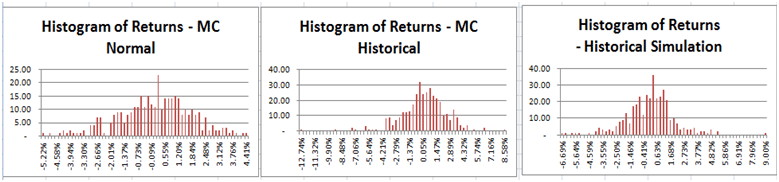
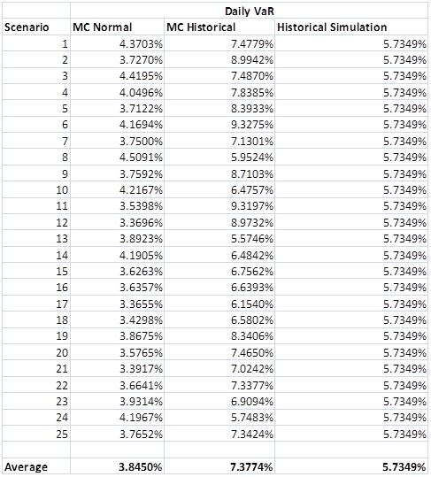
Comparing Monte Carlo Simulation Models & Methods – Gold Prices & Value at Risk Estimates.
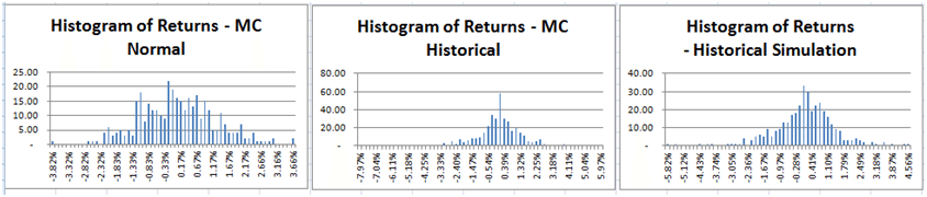
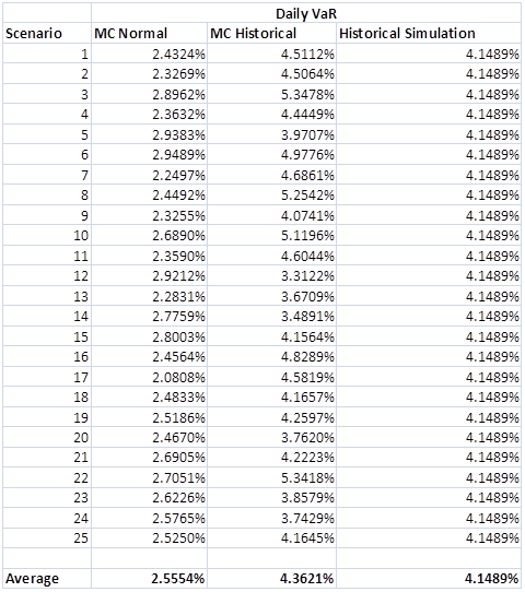
The histogram of returns for the Monte Carlo simulation model that uses the normally scaled random numbers has a much narrower dispersion of values around the mean and does not capture the level of extreme events seen in the gold price series over the past years. Value at Risk (VaR) from the Monte Carlo simulation using the historical returns reflects these extreme events in its tails. Across the 25 scenarios shown above the daily VaR number using the MC – Historical approach is more in line with the daily VaR number obtained using the Historical simulation approach relative to the daily VaR number from the MC- Normal approach.
Note: For the Gold MC model we have assumed an initial spot price of USD 1,657.50 (as at 28-12-2012), an annualized volatility of20.90% (for 2012 daily price returns, a risk free rate of0.16% (I year US Treasury yield curve rates as at31-12-2012) convenience yield of 0%.
Comparing Monte Carlo Simulation Models & Methods – Silver Prices & Value at Risk Estimates.
Note: For the Silver MC model we have assumed an initial spot price of USD 30.15 ((as at 28-12-2012), an annualized volatility of of34.83% (for 2012 daily price returns, a risk free rate of0.16% (I year US Treasury yield curve rates as at31-12-2012) convenience yield of 0%.
Comparing Monte Carlo Simulation Models & Methods – Crude Oil WTI Prices & Value at Risk Estimates.
Note: For the Crude MC model we have assumed an initial spot price of USD 90.91 ((as at 27-12-2012), an annualized volatility of of31.37% (for 2012 daily price returns, a risk free rate of0.16% (I year US Treasury yield curve rates as at31-12-2012) convenience yield of 0%.
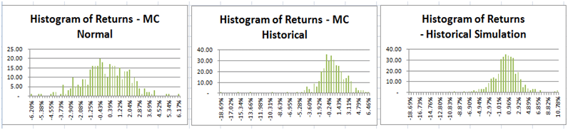
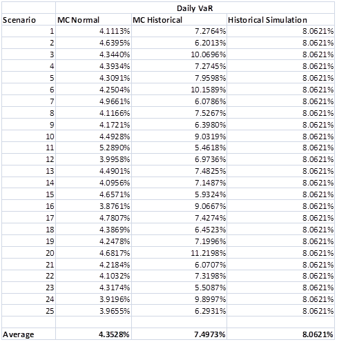
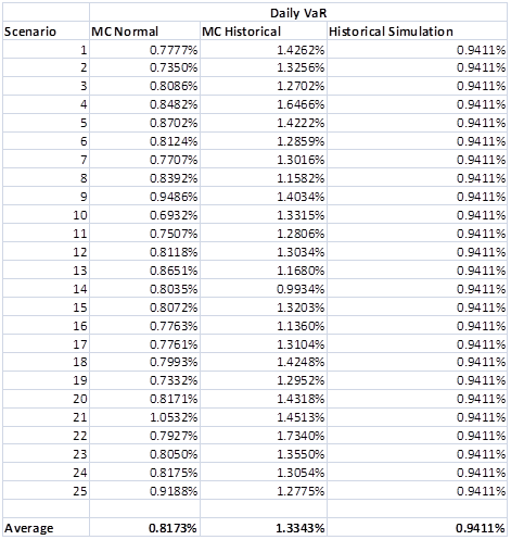
Comparing Monte Carlo Simulation Models & Methods – EUR-USD Exchange Rate & Value at Risk Estimates.
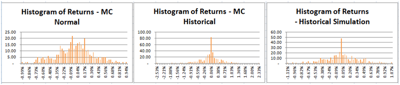
Note: For the EUR-USD MC model we have assumed an initial spot EUR-USD exchange rate of 1.3215 ((as at 31-12-2012), an annualized volatility of of6.73% (for 2012 daily price returns, a USD risk free rate of0.16% (I year US Treasury yield curve rates as at 31-12-2012) and a EUR risk free rate of 0.44% (1 year Euro Libor rate as at 31-12-2012).
In general, the VaR calculated using the MC- Historical approach is more in line with VaR derived using the Historical simulation method, sometimes producing even more conservative results. The latter happens because of the wider window used for determining indexed rates that are used to determine the uncertain component, zt, of the MC – Historical model, in relation to the 1-year window used for the Historical simulation approach.