Have you ever wondered what Value at Risk (VaR) numbers would look like across the same dataset but using the different calculation approaches? In today’s VaR Excel spreadsheet walkthrough session we will do just that. We will demonstrate how to calculate VaR in EXCEL using SMA VaR, EWMA VaR, Variance Covariance VaR, Historical Simulation VaR and Monte Carlo Simulation VaR. We will then dig deeper and calculate incremental VaR, marginal VaR and conditional value at risk. And before we close we will take a short stab at the probability of shortfall.
Basic portfolio construction
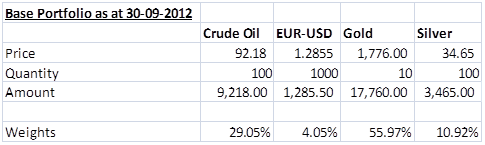
Consider a portfolio comprising of positions in the following:
Figure 1: Investment Portfolio
We aim to calculate VaR using the following approaches:
Variance Covariance Approach
Historical Simulation Approach
Monte Carlo Simulation Approach
You may like to refresh your memory regarding the description and basic mechanics of each approach by taking some time first to look at the following posts before proceeding ahead:
In addition to going through these approaches, we will also look at other VaR related risk measures such as:
Incremental VaR which measures the impact of small changes in individual positions on the overall VaR.
Marginal VaR which measures how the overall VaR would change if we remove one position completely from the portfolio.
Conditional VaR that measures the mean excess loss or expected shortfall beyond VaR at a given confidence level.
Probability of Shortfall which measures the probability that investment returns will not reach a given goal. Alternatively, the probability that investment returns will fall below a given goal.
Preliminary steps
For this exercise we have obtained data for WTI, EUR-USD exchange rate, Gold and Silver for the period January 2004-September 2012 from EIA, OANDA, onlygold.com and kitco.com respectively.
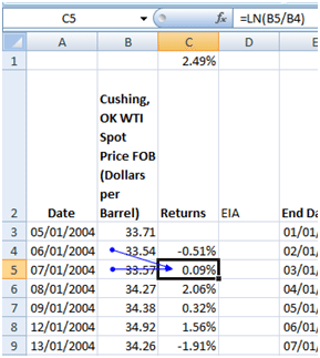
Before we move on to the specifics of each approach we will determine the return time series for each position. Obtain this is by taking the natural logarithm of successive prices. This return series is the foundation for all the methods (except Monte Carlo simulation) and metrics mentioned above:
Figure 2: Calculating return series for each position
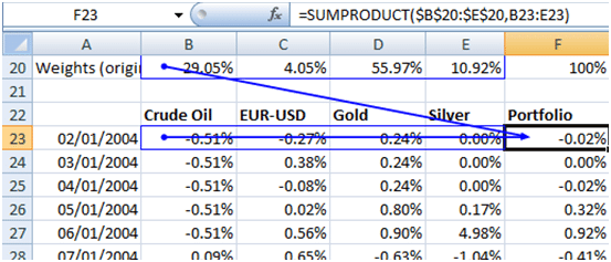
We will also determine the portfolio return series. As you may recall, this return series is a correlation adjusted series. A series that takes into account the correlation between the various positions in the portfolio. Using the weights of each position with respect to the portfolio we calculated a weighted average sum of the returns for each point in time:
Figure 3: Calculating portfolio return series
VaR Approaches
1. Variance Covariance (VCV) Approach
This method assumes that the daily returns follow a normal distribution. The daily Value at Risk is simply a function of the standard deviation of the positions return series and the desired confidence level.
Within the approach sigma may be calculated in two ways:
a. Simple moving average volatility
Using a simple moving average (SMA) approach which places equal importance on all returns in the series. Using EXCEL, determine sigma by using the STDEV function on the array of return series.
Figure 4: Calculating daily SMA volatility
b. Exponentially weighted moving average volatility
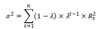
Using an exponentially weighted moving average (EWMA) approach determines sigma as Depending on the lambda chosen greater emphasis may be placed on more recent durations as compared to the SMA approach.
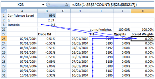
We start of by specifying a value for lambda. The smaller the value of lambda the greater is the weight that is applied to more recent observations. We have used a lambda of 0.5.
Next, we determine the weights Depending on the sample size used the weights may need to be scaled so that the sum of weights equals one. We achieve scale by dividing each weight by 1-(lambda^n).
Figure 5: Calculating weights for determining EWMA volatility
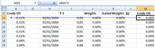
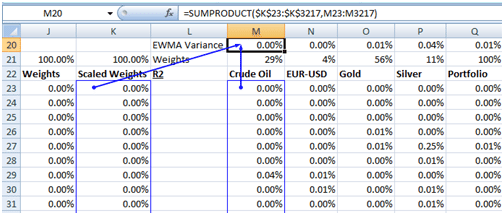
Determine the EWMA variance by taking the weight average sum of the weights and the squared returns as given in the formula above.
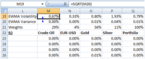
Determine the EWMA volatility by taking the square root of the resulting variance.
Figure 8: Calculating EWMA volatility
c. Final steps & comparison of SMA & EWMA
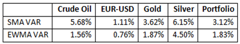
Once we have obtained daily volatility we determine the daily VaR. This is the product of the volatility and the inverse of the standard normal cumulative distribution for a specific confidence level. For a confidence level of 99% the inverse z-score works out to 2.33. The results for the VCV SMA and VCV EWMA approaches are as below:
Figure 9: SMA & EWMA VaR
2. Historical Simulation VaR Approach
Historical simulation is a non-parametric approach for estimating VaR. The returns are not subjected to any functional distribution. Estimate VaR directly from the data without deriving parameters or making assumptions about the entire distribution of the data. This methodology is based on the premise that the pattern of historical returns is indicative of future returns.
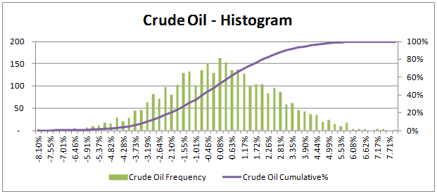
We use the histogram of returns to determine daily VaR. Use the EXCEL Data Analysis histogram function directly on the calculated return series. Alternatively, you may derive the histogram yourself as follows:
a. Step by Step guide to deriving a histogram
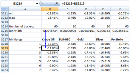
Calculate a minimum and maximum return of the return series
Calculate the width of each bin for the histogram. This will be the difference between the minimum and maximum divided by the number of bins or buckets that you want to use. We had used 60 buckets.
Calculate the bin range values as: bin (1) = minimum value of return, bin (t) = bin (t-1) + bin width
Figure 10: Determining bin range values for histograms
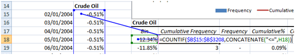
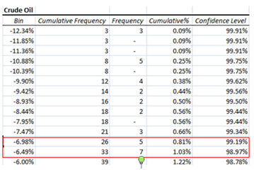
Determine the Cumulative Frequency, i.e. the number of returns that fall with the specified bucket. Using the COUNTIF EXCEL function we determine the number of returns that are less than or equal to the bin value:
Figure 11: Calculating Cumulative Frequency
Determine Frequency for Bin (t) as Cumulative Frequency (t) less Cumulative Frequency (t-1)
Calculate Cumulative % as Cumulative Frequency/ total number of return observations
Determine Confidence Level as 1-Cumulative Frequency
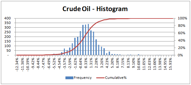
Figure 12: Histogram of historical Crude Oil price return series
b. Calculate VaR
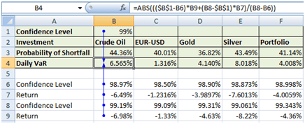
Determine the VaR value that corresponds to a specified confidence level. For example for a confidence level of 99% the VaR will be the interpolated value between -6.98% and -6.49%, i.e.6.565%.
Figure 13: Daily historical simulation VaR
3. Monte Carlo Simulation Approach
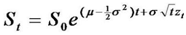
The approach is similar to the Historical simulation method described above except for one big difference. A hypothetical data set is generated by a statistical distribution rather than historical price levels. The assumption is that the selected distribution captures or reasonably approximates the price behavior of the modeled securities. For illustration purposes only we have used the Black Scholes terminal price formula, as our Monte Carlo simulator.
We have replaced mu by r, the risk free rate of 1%, used the annualized scaled daily SMA volatility as our estimate of sigma and taken the initial spot price to be the price available at the end of the period of analysis.
However, for this method to be applied in practice, we need to select a model that is able to explain the behavior of that position’s price over time so that the simulated distribution of values converges to the true distribution of values of the positions and portfolio.
Figure 14: Histogram of simulated Crude Oil price return series
Create the Monte Carlo VaR model using the following steps:
Generate randomly simulated prices
Calculate the daily return series including the portfolio return series.
Determine daily VaR as per the historical simulation histogram approach
Repeat the above three steps a large number of times. Utilize EXCEL’s Data Table functionality to generate a table of results for each simulated run.
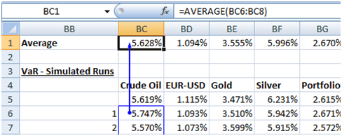
Calculate the average VaR across all simulated runs
Figure 15: Average MC simulated Daily VaR across all simulated runs
a. Results Summary
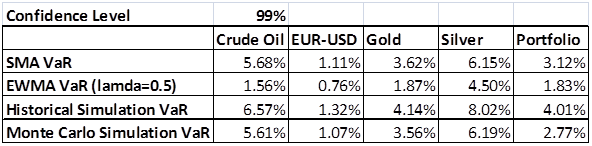
Here is the summary of results from all the approaches:
Figure 16: Summary of results from all approaches
VaR Related Risk Measures
1. Incremental VaR
Incremental VaR (IVaR) measures the impact of small changes in individual positions on the overall VaR. There are two different approaches to calculating incremental VaR:
Full valuation approach
Approximate solution to IVaR or the short cut approach
a. Full valuation approach
In the Full valuation approach the entire process for VaR is repeated based on the revised positions of the portfolio. This means that we are calculating the VaR value twice. Incremental VaR will be the difference between the original VaR calculation and the revised VaR calculation.
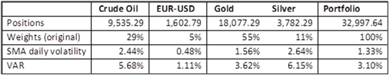
Let us review our portfolio once again:
Figure 17: Investment Portfolio
The total portfolio value works out to 31,728.50. The SMA daily VaR is 3.12%. The portfolio VaR amount worked out 31728.50*3.12% = 991.23
Assuming a 1% increase in all positions with respect to the total portfolio value the revised portfolio (all position increase by 317.285) will be as follows:
Figure 18: Revised Portfolio values, weights, volatility and VaR
The revised portfolio VaR works out to 32997.64*3.10% = 1023.89
The incremental VaR, therefore, is 32.66.
This process may not seem too tedious with just 4 positions. However, a financial institution may have a portfolio comprising of hundreds of different positions. This could make the full valuation process time consuming.
There is however a short cut solution to IVaR that does not require two separate VaR valuations.
b. Approximation to IVaR
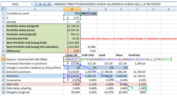
The incremental VaR using the short cut method is approximately equal to:
Absolute value of (Change in position relative to original portfolio value *Original Portfolio Value) * inverse z-score of selected confidence level * Covariance between original position returns & original portfolio returns/ Original Portfolio volatility.
Figure 19: Calculation of IVaR using the approximate method
If you look at the above formula you will notice that we have attached a condition on the calculated Covariance. If we are long on the original position and the incremental position is an increase in the position or if we are short of the original position and incremental position increases the short position then we take the covariance as is. However, if we are long on the original position and the incremental position is a decrease in the position or if we are short of the original position and incremental position decreases the short position then we take the covariance as -1*covariance.
Using the approximate method we arrive at an incremental VaR of 32.58. This is 0.09 less than the IVaR figure derived using the full valuation approach.
Note: The Covariance for the EWMA VaR approach is calculated as the sum product of the following series:
the return series of a given position,
the return series of the original portfolio, and
the scaled weights.
2. Marginal VaR
Marginal VaR measures how the overall VaR would change if one position was completely removed from the portfolio.
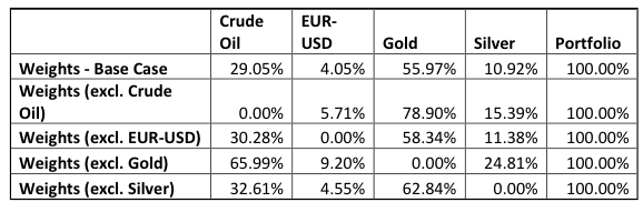
As the first step in this process we determine the weights of the portfolio assuming all four positions are present and then again if one position (at a time) were to be eliminated as follows:
Figure 20: Portfolio weights – original and revised positions
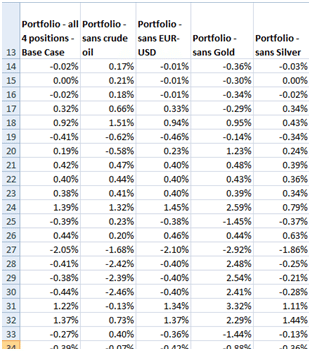
Next, we recalculate the portfolio return series using the revised weights as follows:
Figure 21: Portfolio returns – original and revised series
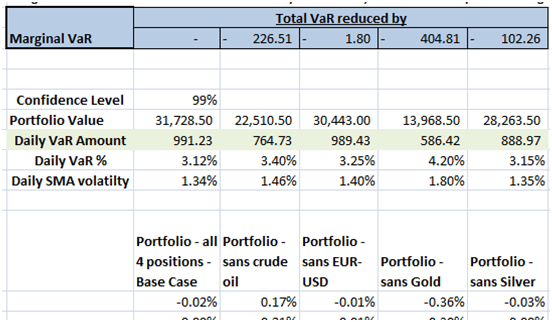
We then recalculate the volatility, VaR % and VaR amount based on the revised return series:
Figure 22: VaR – original and revised values
The marginal VaR, if we remove crude oil from the existing portfolio, is 226.51. The VaR amount will reduce by this figure. Note that in % terms portfolio VaR has increased but the portfolio value to which the VaR% applied has reduced hence there is a reduction in the overall VaR amount.
3. Conditional VaR
Conditional VaR measures the mean excess loss or expected shortfall beyond VaR at a given confidence level.
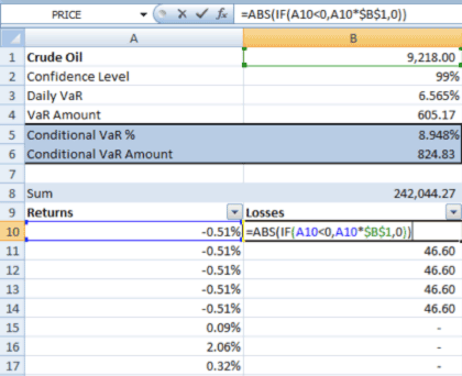
For our illustration purposes, we assume that VaR % has been calculated using the Historical Simulation approach. Calculate the VaR amount is as VaR % * Portfolio or Position Value.
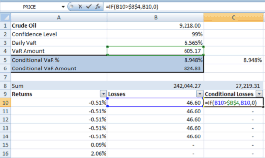
For each data point we first calculate the amount of loss which is the Portfolio or Position Value * Return. If the return is negative it will be taken as a loss whereas if it is positive zero losses will be recorded.
Figure 23: Loss amounts
We next determine the conditional losses. In effect, this is the loss amount already calculated above but subject to a restricting condition. Only those losses than exceed the VaR amount will be considered:
Figure 24: Conditional loss amounts
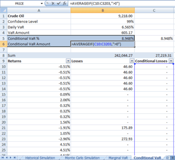
We next calculate a weighted average VaR % where the weights are based on the conditional losses. Calculate this as the sum product of the Returns times the Conditional Losses. Then divide the result by the sum of the Conditional Losses. This average VaR% is the Conditional VaR %. Multiply with the portfolio or position value to arrive at the Conditional VaR amount or the average loss amount assuming that it is in excess of VaR.
Figure 25: Conditional VaR
4. Probability of Shortfall
Probability of Shortfall measures the probability that investment returns will not reach a given goal or alternatively the probability that investment returns will fall below a given goal. For illustration purposes, we assume that our goal is that position or portfolio returns should never be negative. They should be greater than zero.
Given our distribution of returns what is the probability that returns will be negative?
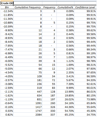
Using the histogram methodology of the Historical Simulation approach we have already determined the cumulative frequency of returns being less than or equal to a particular value. We just need to identify this cumulative frequency for returns less than or equal to 0%.
Figure 26: Evaluating the probability of shortfall for crude oil from the histogram table
For Crude Oil we can see that the probability that returns will be negative is 44.36%.
For the other positions the probability of shortfall is as follows:
Please review the file description to confirm if this is what you are looking for before proceeding with the purchase.
Regards
FinanceTrainingCourse.com
I would like to know where from I can get data associated with RiskMetrics. The riskmetrics doc says that it is freely available but I could fetch from Web. Kindly guide me.


Hello,
Is there somewhere I can find the example´s excel sheet ? is it available for dowload?
thanks a lot
best regards
Dear Martin,
Thank you for your interest in our post “Value at Risk (VaR) models, methods & metrics – Excel spreadsheet walk through”.
We do have an EXCEL sheet available for purchase – Comparing Value at Risk – Model, Methods and Metrics – EXCEL at the store under the “RISK MANAGEMENT” category at the following link http://financetrainingcourse.com/store/#!/~/product/category=1944018&id=17285013.
Please review the file description to confirm if this is what you are looking for before proceeding with the purchase.
Regards
FinanceTrainingCourse.com
I would like to know where from I can get data associated with RiskMetrics. The riskmetrics doc says that it is freely available but I could fetch from Web. Kindly guide me.