You are interested in creating your own investment portfolio. What are the elements or factors that you should consider when putting it together? In finance, there are two main pricing theories for valuing or assessing portfolios. The first one is the Capital asset pricing model (CAPM). This model relates expected return to a single market wide risk factor. By contrast the second theory, the arbitrage pricing theory (APT), relates returns to either multiple factors that impact market wise risk such as macroeconomic factors like money supply, inflation, GDP or multiple proxies that explain the risk premium over the risk free rate such as excess market return, firm size, book value to market value ratio, price to earnings ratio, financial leverage, etc. In this post, we focus on capital asset pricing model (CAPM) for determining & valuing our potential investment portfolio.
a. Laying the foundation – key statistical measures
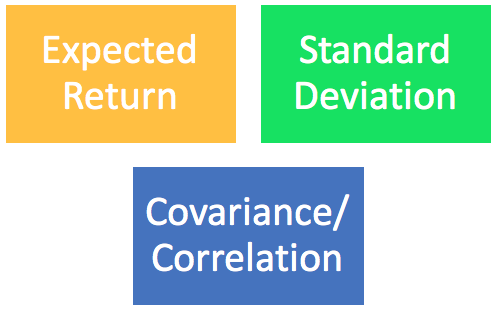
Capital asset pricing model (CAPM) builds on the capital market theory which in turn extends the Markowitz portfolio theory. The foundation of these three theories are the following statistical measures:
Expected return, assessed using historical returns of a given security, is the probability weighted average return. For example, the price history of stock ABC reveals that 60% of the time the return was 10% whereas for the remaining 40% the return was 5%. The expected return for ABC, therefore works out to 60%*10% +40%*5% = 8%.
When using daily returns based on historical series of stock prices, you can create a histogram of returns to determine the probability distribution for the return series and estimate the expected return. Equivalently you can assume that each return has an equal probability of occurring, i.e. a probability of 1/No of returns observations in the historical window selected.
Using the AVERAGE () function in EXCEL across the daily return series would result in the same value.
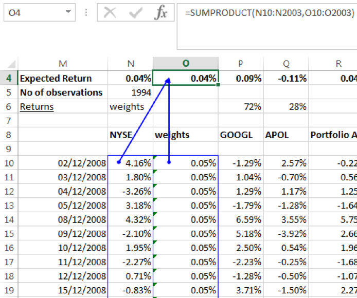
The expected return for a portfolio is simply the weighted average expected returns of the individual securities in the portfolio where the weights are the investment’s value in relation to the portfolio value. Alternatively, it may be derived from the returns series of the portfolio where returns are the weighted average of the individual asset returns.
Variance or standard deviation measures the volatility of the returns from the expected return. For an individual security it may be calculated using the following formula (shown for a portfolio of three securities) or using the STDEV function in EXCEL across the daily portfolio return series:
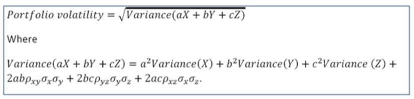
From the above equation is it clear that the portfolio’s standard deviation is a function of the variances and covariance of the individual securities. In particular as the number of securities increases the impact of the covariance element of the formula outweighs that of the variance elements. Knowing the relationship between securities is a critical factor when selecting securities for your portfolio. Choosing the correct relationship could mean, that for a given return we could reduce the risk of the portfolio. We will look at a simple example of this below, but first let us take a closer look at the final foundational measure common to the Markowitz portfolio theory, capital market theory & capital asset pricing model (CAPM), i.e. Covariance/ Correlation.
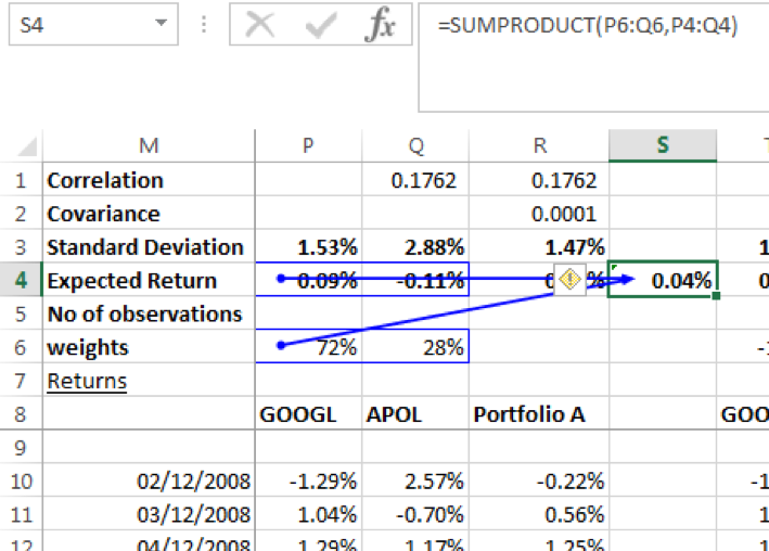
Covariance is a measure of the degree to which a security’s and portfolio’s returns move together in relation to their expected returns. Correlation standardizes the covariance measure, by dividing the covariance with the security & portfolio’s standard deviations, so it falls between -1 and +1. If negative, returns of the security and portfolio move in opposite directions to each other relative to their expected returns; if positive they move in the same direction. A zero value indicates no correlation, while a value close to +1 or -1 indicates high correlation.
Let us consider the following portfolio of two securities GOOGL & YHOO. Both are technology search engine company stocks. We would expect them to be positively correlated. Given the dataset we have used, the returns are moderately positively correlated with correlation coefficient = 0.4139. GOOGL has an expected daily return of 0.090% whereas YHOO has one of 0.067%. With weights of 15% and 85% respectively the expected return of the portfolio is 0.070%, and standard deviation is 1.79%.
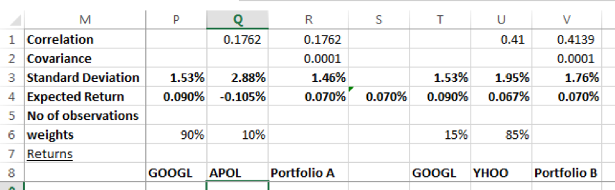
What happens when we replace YHOO with APOL in the portfolio? APOL an education system company has a negligible correlation with GOOGL of 0.1762. APOL expected daily return is -0.105%. Choosing positions of 90% and 10% respectively for GOOG & APOL to achieve the same portfolio return of 0.070%, we see than the lower correlation has effectively reduced risk to 1.46% a 33 basis points reduction.
b. Markowitz portfolio theory
The Markowitz portfolio theory formally developed expected return and risk measures for portfolios of assets and showed how to use the relationship between securities returns to diversify away and reduce portfolio risk to obtain an efficient set of portfolios called the efficient frontier of risky assets. The efficient frontier represents the best and most efficient combinations of risk and return, i.e. maximum expected return for a given level of risk or minimum risk for a given return.
Assumptions
The theory itself is based on a number of assumptions on investor’s behavior:
- Investments are represented by a probability distribution of expected returns over some holding period (daily, weekly, monthly)
- Risk is assessed from the variance of expected returns
- Decisions are solely based on risk-return trade offs
- Investors prefer higher returns over lower returns for a given risk level and lower risk to higher risk for a given expected return
- Investor seeks to maximize their one-period utilities where their utility functions have diminishing marginal utilities of wealth
Efficient frontier
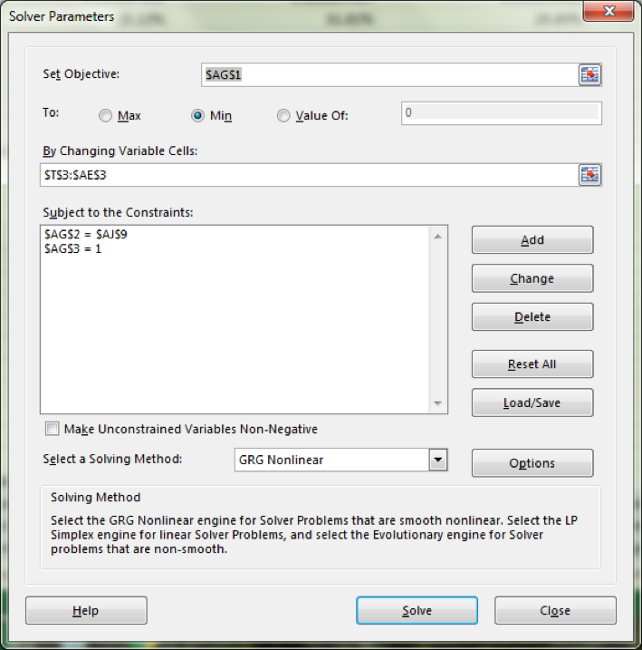
Let us assume that the universe of risky assets consists of the only 12 stocks. The efficient frontier of risky portfolios can be constructed by minimizing the variance for any targeted expected return. The calculated annualized portfolio standard deviation (Cell AG1) is minimized by changing the portfolio weights across the securities (Cells T3-AE3) while ensuring that the sum of weights is equal to 100% (Cell AG3) and the expected annualized return (AG2) equals the targeted expected return (AJ3 to AJ22 in turn). This assumes that short sales and fractional positions are possible. If certain markets restrict such transactions additional constraints may be added to the variance minimization model and the resulting efficient frontier will be different.
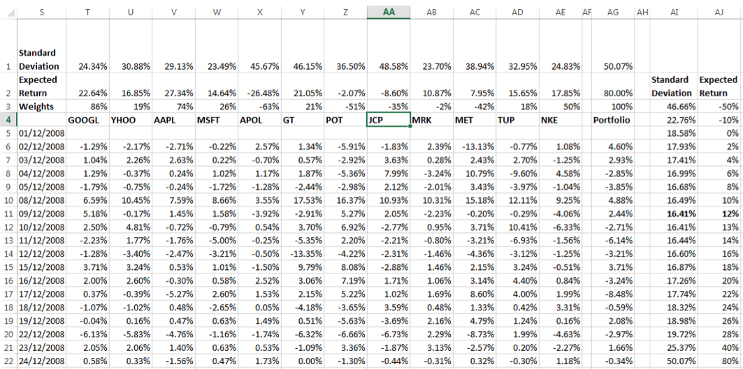
In EXCEL the solver function can be used for this optimization process.
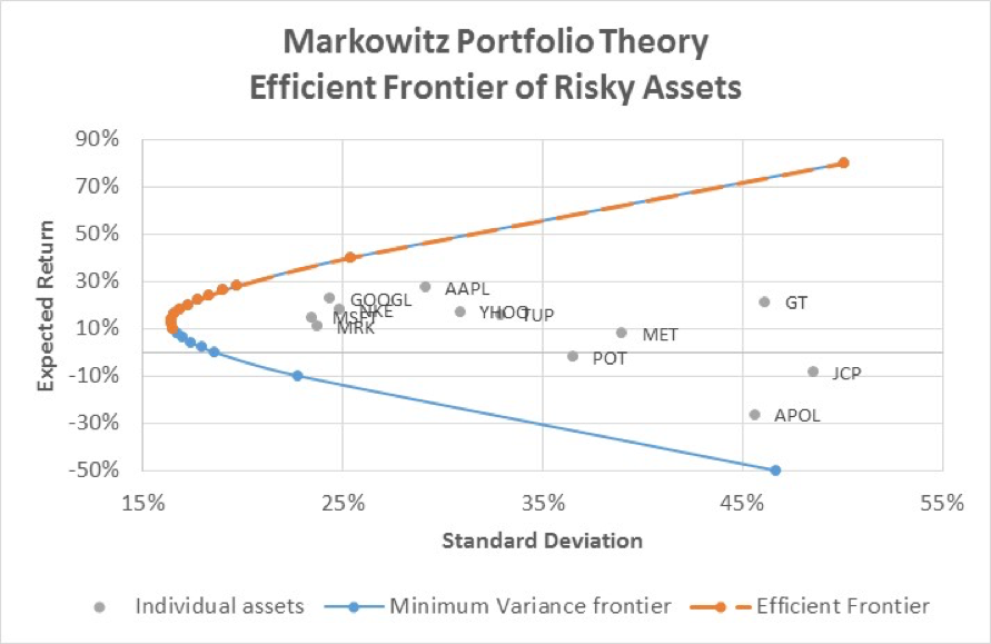
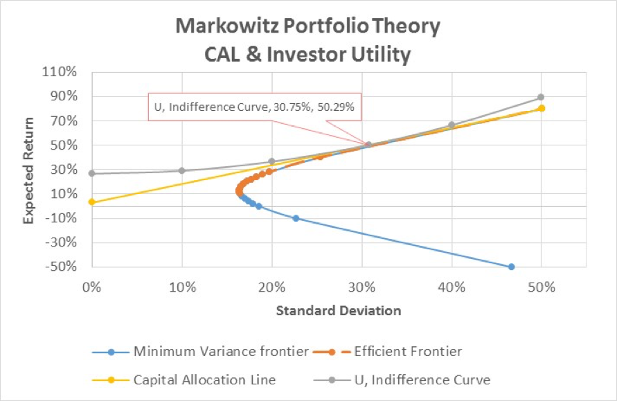
The resulting graph gives the minimum variance frontier, where the top portion of the curve (highlighted in orange) shows the efficient frontier. The bottom portion of the minimum variance curve is not efficient as for a given standard deviation there is a higher target expected return possible.
Individual asset risk- returns lie within the area marked off by the efficient frontier.
c. Capital allocation line
Once we have the efficient frontier of risky assets we need to determine which risky asset portfolio on the curve is the optimal one. This is the portfolio that will provide us with the highest reward-to-variability ratio which is given by the following equation:
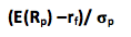
Where
rf is the rate of return on a risk free asset
E(Rp) is the expected rate of return of the risky asset portfolio
σp is the standard deviation of the rates of return of the risky asset portfolio relative to the expected rate of return
This is also the slope of the investor’s capital allocation line (CAL), i.e. the line representing the feasible combinations of risk-return available to the investor – his investment opportunity set. The investor’s best combination from the feasible options will depend on his level of risk tolerance, which will dictate the proportion of investment budget he will allocate to the risk free asset and to the risky asset portfolio, and his position on the CAL.
In our example, we assume a risk free rate of 3%. The optimal risky portfolio (P) with the highest reward-to-variability ratio is at expected return = 80% and standard deviation of 50.07% (ratio = 1.54). Our CAL is the straight line from the risk free rate on the Y axis to point P, which is tangent to the efficient frontier as graphed below:
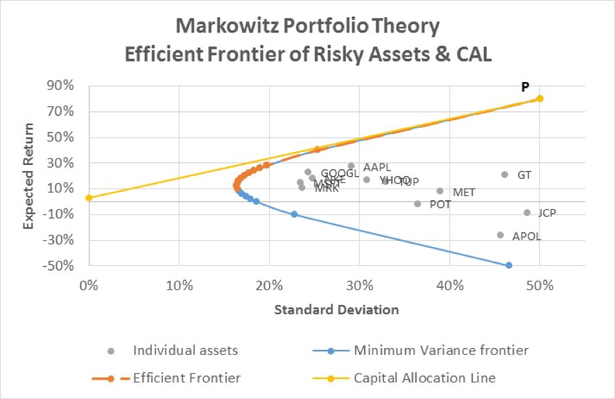
Note: The CAL is superimposed on the EXCEL graph of the efficient frontier by adding a series to the graph for the following values:
| σ
(x-axis) |
E (R )
(y-axis) |
| 0.00% | 3.00% |
| 50.07% | 80.00% |
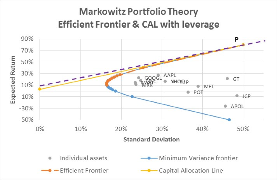
Risky asset portfolio options to the right of P, if the straight line is extended beyond P, are leverage opportunities with higher return for higher risk, if the investor can borrow at margin and invest additional proceeds into the risky asset portfolio. This would only be possible if the investor could borrow at the risk free rate, which for most investors unless they are sovereign entities, is not the case. For non- government investors the CAL line beyond P would be kinked to show that any borrowing for leveraging return would be based on a higher rate than the risk free rate (the purple dotted line):
Utility and the investors’ indifference curve
Different investors will choose different combinations of the risky asset portfolio and the risk free asset based on their degree of risk aversion which is graphically captured in their utility function or indifference curve. One common representation of utility is the equation:
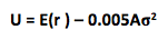
Where U is the utility value and A represents the investor’s degree of risk aversion. Higher As are assigned to more risk averse investors who penalize higher riskiness (as indicated by the variance measure). The indifference curve is a combination of portfolio choices that represent equal utility for the investor given his level of risk aversion.
In relation to CAL the investor will choose that combination of risky portfolio to risk free asset that will optimize his utility. The combination chosen is known as the investor’s complete portfolio.
If the proportion invested in the risky portfolio is p, then 1-p is the proportion that will be invested in the risk free portfolio. The expected return on the investor’s portfolio, E (r) is a weighted average return of the risk free rate and the risky asset portfolio return:
E(r ) = y(E(Rp)) + (1-y) rf = rf + y (E(Rp) –rf)
The variance of this portfolio will be:
σ2 = y2σp2
If we put this in our utility function we have:
U = rf + y (E(Rp) –rf) – 0.005A y2σp2
If we maximize utility U (by taking the derivative of U with respect to y and setting the resulting equation to 0) and solve for y we get:
y%= (E(Rp) –rf)/(0.01Aσp2)
Let us assume that our investor has a risk aversion of A = 5. Given our expected return and risk of the optimal risky asset portfolio of 80% and 50.07% respectively, the proportion that the investor will allocate to the risky asset portfolio is:
y% = (80% -3%)/(0.01*5*50.07%^2) = 61.4168%
The expected return & standard deviation of the chosen complete portfolio for the investor will therefore be:
E(r ) = y(E(Rp)) + (1-y) rf = rf + y (E(Rp) –rf) = 3%+0.614168*(80%-3%) = 50.29%
σ = √(y2σp2) = yσp= 0.614168*50.07% = 30.75%
This portfolio is graphically depicted below as the point where the CAL forms a tangent to the investor’s indifference curve, U.
Note: The utility curve has been imposed on the efficient front and CAL in the EXCEL graph by adding a series for the indifference curve. This series is determined by first calculating the utility of the investor’s optimal portfolio using the expected return and the standard deviation derived above, i.e:
U = E(r ) – 0.005Aσ2 = 26.65%
Holding this utility constant as the investor will have the same utility across the indifference curve, rearranging the equation above to solve for expected return and varying the standard deviation we determine our indifference curve series as follows:
| σ (x-axis) | 0.00% | 10.00% | 20.00% | 30.75% | 40.00% | 50.00% |
| E(R ) (y-axis) | 26.65% | 29.15% | 36.65% | 50.29% | 66.65% | 89.15% |
d. Capital Market Theory
The capital market theory is an extension of the Markowitz Portfolio Theory.
In the capital market theory, the efficient frontier represents well diversified (as to unsystematic or specific risk) portfolios of all risky assets, not just any portfolio of risky asset.
The tangent to the curve is at a market portfolio that has the highest reward-to-variability ratio as compared to all other well diversified portfolios on the efficient frontier. This tangent is the best capital allocation line.
In this instance, the CAL is known as the Capital Market Line (CML). It shows combinations of the investment or borrowing in a risk free asset (e.g. one month T-Bills) with the optimal well diversified market portfolio (e.g. a broad based market index). It is given by the equation E(Rp) = rf + σp(E(RM) – rf)/ σM, where M is the optimal well diversified market portfolio containing all risky assets at the point of tangency of the efficient frontier and the CML.
Because the market portfolio is well diversified, σM & σp both are comprised only of non-diversifiable systematic risk.
The investor’s complete portfolio is represented by the tangent of his indifference curve to the CML. This would represent his optimal allocation between the risk free asset and the well diversified portfolio based on the maximum utility derived from such a portfolio given his degree of risk aversion.
Assumptions
This theory and capital asset pricing model (CAPM) are based on a number of simplifying assumptions on investor behavior:
- The market consists of many investors with individual investor wealth that is a small portion of total wealth across all investors, and whose individual trades will not impact asset prices
- All investors plan for the same single holding period
- All lending and borrowing are at the risk free rate, and investments are made in publicly traded financial assets only
- There are no taxes or transactions costs on trades
- All investors want to maximize expected returns for a given level of risk or minimize variance for a given level of return
- Investors have homogeneous expectations. They analyze data the same way so that their expected returns, variances and covariance and hence efficient frontier and optimal risky portfolio on that frontier, will be the same for a given asset data set.
e. Capital Asset Pricing Model
Capital market theory uses total volatility (σ) in the determination of the portfolio return and risk. However, in the market, investors are only compensated for systematic risk, i.e. risk that cannot be diversified away, such as those risks arising from macroeconomic factors such as a rise in inflation, a fall in production, etc. They do not get paid for unsystematic, company specific risk as this can be reduced with effective portfolio management. The use of total volatility in determining expected portfolio return and its variance is only appropriate for evaluating the risk and return trade-offs for fully diversified portfolios as the total volatility represents only systematic risk. The capital market line cannot be used to assess the risk return trade-off for undiversified portfolios or individual assets where the total volatility comprises of both systematic and unsystematic risk.
Using the CML for individual assets or undiversified portfolios, in particular, the total volatility measure would result in an overestimation of their expected returns and risk.
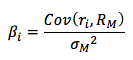
Capital asset pricing model (CAPM) resolves this issue, and generalizes market theory for individual securities, by replacing total risk of the portfolio in relation to the market risk with a measure of systematic risk in relation to the market risk, i.e. Beta given by the formula:
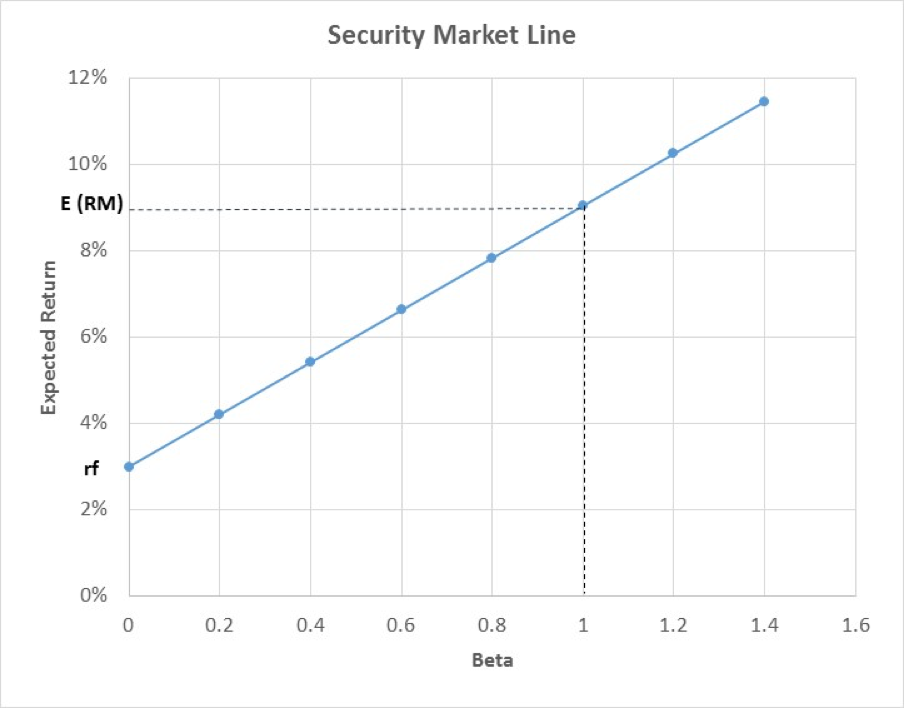
The expected rate of return is given by E(ri) = rf + βi(E(RM) – rf) and is known as the security market line (SML). Under capital asset pricing model (CAPM), SML can be used for assessing risk return trade-offs for both well diversified portfolios as well as individual assets.
For individual assets, the SML gives the risk premium of the asset relative to its risk. M represents a well-diversified market portfolio and beta represents the asset’s contribution to that portfolio’s risk.
Let us assume that our well diversified market portfolio is represented by the NYSE index.
(Note: NYSE is not a truly diversified portfolio as it is only an index of stocks and not the full universe of risky assets, but for the sake of illustrating the use of SML we have used it as our market portfolio.)
The annualized expected rate return and volatility of returns for NYSE based on index price data from 1-Dec-2008 to 1-November-2016 is 9.04% and 19.01% respectively.
Using the SML equation we can plot the line for varying beta (the blue line in the graph below). For example, the required expected return for a beta of 1 and a risk free rate of 3% works out to:
E(ri) = 3% + 1 * (9.04%-3%) = 9.04%
A beta of 1 means E(ri) represents the market portfolio’s expected return, E(RM) = 9.04%.
For a beta of 0.4, the required rate of return is:
E(ri) = 3% + 0.4 * (9.04%-3%) = 5.42% and so on.
When assets are priced fairly, i.e. when markets are in equilibrium, the estimated rates of return will lie on the SML and match the required rates of return given a level of systematic risk. When assets are not priced fairly or the market is in disequilibrium, estimated rates of return will either lie above or below the SML.
If the estimated rate of return for an asset lies above the SML, the asset is undervalued. The difference between the estimated rate of return and the required rate represents positive alpha or the excess return. If the estimated rate of return lies below the SML, the asset is overvalued, as the required rate for the given level of systematic risk is greater. Alpha would be negative in this case.
We illustrate this for our data set of 12 equity stocks. We estimate the annualized expected return and beta for each of the stocks from the price history for the period 1-Dec-2008 to 1-November-2016 and plot them in the graph containing the SML:
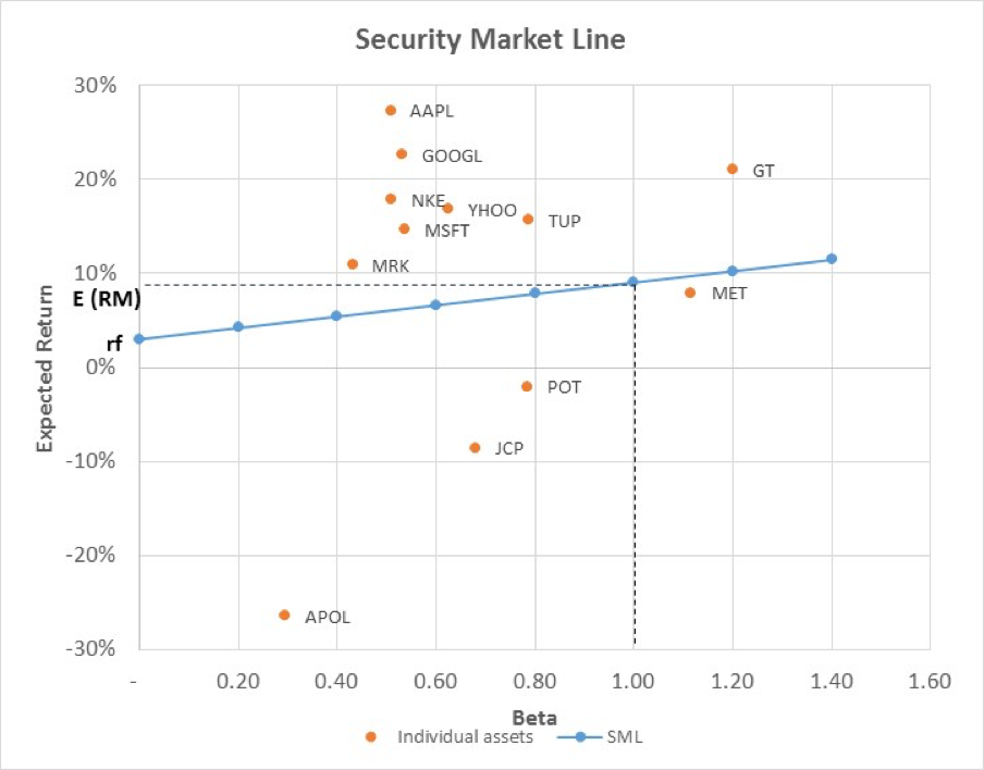
We can see that GOOGL which has a beta of 0.53 has an estimated rate of return of 22.64%. This is higher than the required rate of return given the level of systematic risk of:
E(ri) = 3% + 0.53 * (9.04%-3%) = 6.21% meaning that GOOGL is undervalued and has a positive alpha value of 16.43%.
By contrast, JCP is an overvalued stock given that its beta is 0.68. The required rate of return for taking on this level of risk is 7.10% whereas it has a negative estimated return of -8.60%.
The stock with an estimated return-beta relationship closest to the SML is MET, with an estimated return of 7.95% against a required one of 9.74% for a beta of 1.12. It is slightly over valued with a negative alpha of -1.79%.
References:
- Analysis of investments & management of portfolios – Reilly Brown (10th Edition)
- Investments – Bodie, Kane, Marcus (4th Edition)