How to effectively assess portfolio performance
What is the best way of evaluating portfolio performance allocation strategies? Should we just compare risk, return or risk adjusted return? Are complex investment allocation models and tools more effective than simpler ones? Is one framework better than other? When we look at fund managers or fund performance what data should we seek and collate? How do we know if we one investment strategy is better than the other? What benchmarks can we use to assess how well we have done relative to the market?
All great questions. We answered these and more in the latest iteration of the portfolio management and optimization models course last October in Dubai. Let’s take a look at what we found out.
Experiment design
We used a simple experiment design with a universe of preselected investment securities and 5 investment allocation models. The securities data set looked at prices from 2008 to 2018. 2008-2016 data was used to train allocation models and allocate capital to specific positions. 2016-2018 data was used for evaluating performance of each allocation.
The model increased in their sophistication moving from a simple risk adjusted return approach to more complex designs. Models focused on minimizing probability of loss as well models that focused on increasing the probability of upside by optimizing the distribution of returns.
For performance evaluation we used three benchmarks. Two linked to index performances (NYSE and NASDAQ) and one linked to a security that outperformed all other securities within the portfolio during the observation period (AMZN).
Using historical securities price data, we allocated capital to investment securities. The allocation model had access to prices from 2008 till 2016. Performances were evaluated separately for two periods. 2016-2017 and 2016-2018. The performance metric was holding period return (HPR) which measured total return over the evaluation period. The 2016-2018 evaluation served as a post allocation performance evaluation. We then evaluated their performance by comparing the results against performance of the three benchmarks.
All models used historical return series to allocate capital. This implies that future performance can be projected using historical returns. We understand that this is not true but this is the basis of the original allocation model. Once the optimal allocation strategy is identified it can be tweaked to take into consideration cyclical performance and the impact of product, user, demographic and economic cycles.
Any guesses on which models out performed others. Before you read further take a second to think about the following questions.
- Given two allocation models, one more sophisticated than the other, which one is likely to outperform the other? Simpler over more complex or more complex over simpler?
- Is it possible to maximize upside and limit downside at the same time? Is there a model that would allow us to trade between the upside potential and downside risk?
The distribution of returns
We have spent a great deal of time on understanding how returns distribution are generated in an earlier part of our course on Portfolio Optimization models. If you are not familiar with the concept of returns distribution, how to calculate them or how to plot them using Excel please see building portfolio management worksheets in excel.
Strategies and evaluation benchmarks
Let us take a quick look at the five investment allocation models used in the experiment. The first two allocation models are metric driven. The last three are returns distribution driven. Of the metric driven, the first focuses on return, the second focuses on risk. Of the distribution driven, the first two focus on the down side, the last one focuses on the upside.
Strategy I – base case – Simpler is better. We calculate return per unit of risk and then optimize that as our internal metric. Return is defined as holding period return over a historical observation period. Risk is defined by observed annual standard deviation of daily return over the same period.
Strategy one is essentially a simplified version of the good old Sharpe ratio, one of the oldest portfolio allocation designs that works of two dimensions at the same time – risk and return.
Strategy II – Minimize downside. Represented by worst case single day loss (WCSDL) using historical returns. WCSDL is defined as the minimum value observed in daily price returns for a given security in the observation period. At a portfolio level it is defined as the minimum value in the portfolio return series during the observation period. The optimization model minimizes the portfolio worst case single day loss.
Strategy two is a Value at risk (VaR) based design that sets a simple threshold using historical data set on the worst case possible loss the portfolio return distribution has experienced during the observation period.
Strategy III – Minimize probability of shortfall. Minimize the probability that returns will fall below some threshold. Probability is measured by the distribution of portfolio returns. In the first shortfall model it the loss threshold is set at 5%. The optimization model minimizes the probability that this threshold will be hit by portfolio returns. In simpler words, this means that the portfolio allocation model will focus on reducing the probability of losing more than 5%.
Strategy three come from the shortfall school. The shortfall school is related to the value at risk school but rather than focusing on a single day loss, it focuses on reducing the probability that a loss threshold would be hit.
Strategy IV – Minimize probability of shortfall. Same model as Strategy III. The loss threshold is set 1%. The optimization model minimizes the probability that we will hit a loss of 1%.
Strategy four is the same as strategy three with a lower loss threshold.
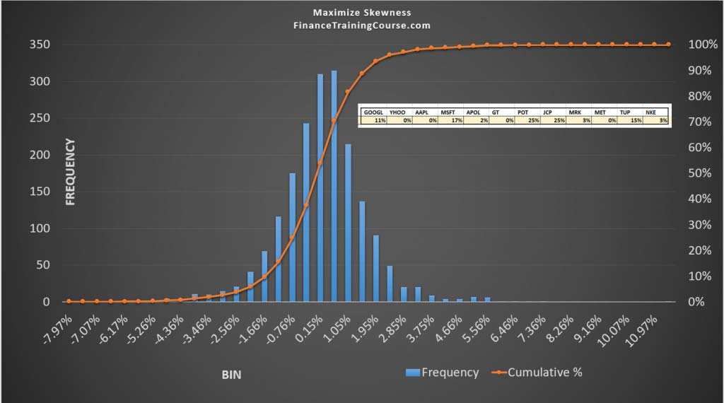
Strategy V – Optimize skewness of returns. Skewness refers to attribute of return distributions that shifts it in a certain direction. Will it help performance if we shift the historical distribution of returns to emphasize positive returns more than negative returns? We test this assumption by maximizing positive skewness of the portfolio return distribution.
Strategy five is the most complex of all five strategies. While strategy two, three and four are also driven by the return distribution, five actually tries to shift the portfolio distribution towards the positive end of return spectrum. The hope is that perhaps doing so we will improve the risk return trade off.
Benchmarks used. NYSE, NASD and AMZN return series over the same period.
Once again before you read ahead, which strategy are you likely to choose as a portfolio manager? Which model do you think out performed all others?
One ring to rule them all?
How well did your chosen strategy perform? Did you expect these results? Were you surprised? Can a deeper dive into performance metrics explain what happened?
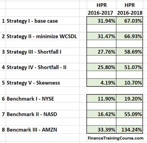
The simplest strategy risk adjusted return, outperformed the more complex one and came very close to beating all three benchmarks in the primary evaluation period. It still dominated all other strategies and 2 of the three performance benchmarks in the post allocation evaluation period that included 2018.

Can you come up with a justification or rationale for these results? Let’s take a look at additional metrics to see if we can find any hints?
The results

The primary performance metric was holding period return or HPR. HPR describes the total realized return over the observation period. It is a better performance metric than expected return or average expected return which is the reason why we used it for performance evaluation.
Our second performance metric was downside as indicated and measured by worst case single day loss. Our third measure was annualized volatility as a measure of risk.
In addition to these other metrics of notes that were tracked across strategies were Beta and Alpha with respect to NYSE (Dow Jones) index, percentile returns at the 1% threshold, maximum single day gain, skewness and kurtosis of the portfolio return distribution.
Take a minute to compare the metrics shared above with post allocation performance for each strategy. Is there anything that stands out?
Here is a hint. In your opinion which attributes highlighted above are the strongest predictors of future portfolio performance?
Risk adjusted returns
The answer once you take a deeper look at the figures is risk adjusted return. Changes in expected return, volatility, beta, worst case single day loss or max single day gain are not sufficient enough to attribute changes in expected performance as well as risk adjusted return does. The same also holds true for percentile returns, skewness and kurtosis.
Alpha is a special animal. While it appears that it may have the same predictive powers as risk adjusted return, we have to be a little careful with this assumption. Take a look at our discussion around alpha cyclicality and optimal portfolio alpha allocation before you commit to alphas as your primary performance metric.
Implication for portfolio managers?
One, if you don’t have a fancy performance monitoring dashboard that is fine. You just need risk adjusted return or what is commonly known as the good old Sharpe ratio.
Two, as you move to more sophisticated approaches or attempt to limit downside, you also limit your upside. Theoretically speaking maximizing positive skewness has a great deal of technical appeal.
It maximizes upside by shifting the returns distribution in the positive direction. If you take a look at the maximum single day gain row, you will notice that maximizing skewness has the highest score for that metric. But what impact does that have on expected return and realized holding period return? As you limit your downside, you will by definition limit your upside.
Three, it appears that there is a clear trade off and no arbitrage possible between the two extremes. At least within this data set. You could change the securities universe and try again but results would remain similar. Sounds counter intuitive but it is true.
Whatever you save in terms of downside you will end up giving up in upside. A distribution of returns comes with a certain amount of risk. The two are linked, you can’t have more of one without having more of the other.
For instance, when we push positive skewness higher, even though we increase the maximum single day gain, we also increase returns volatility and we end up reducing holding period return by a fairly significant amount.
Then why bother with all the metrics?
The metrics are useful when it comes to exploring performance and to answer question posed above. If you want to compare capital allocation strategies, you want to compare them across multiple dimensions not just one. When it comes to designing performance evaluation systems, you want to focus on the one metric that the organization needs to optimize. One that is simple, effective and relevant. While you may understand that simpler is better, you still need good data to convince the world that your baseline model does outperform the more sophisticated editions.
Conclusions and takeaways
Remember the questions we asked above right at the start. Let’s try and answer them one by one
Should we just compare risk, return or risk adjusted return?
Risk adjusted return leads to better performance than just optimizing risk or return. It beats all other benchmarks because they focus on one dimension – risk or return. Risk adjusted return work with two – risk and return.
Are complex investment allocation models more effective than simpler ones?
They can certainly do a better job of limiting downside but there is a cost. In terms of actual performance measured in terms of realized returns, they don’t perform as well as simpler metrics. That is because as you reduce risk beyond a certain threshold, you also reduce the potential for higher returns. Nothing illustrates this more powerfully than the positive skewness strategy in the example above.
Is one framework better than other?
That depends on what you want to measure and achieve and what metrics and benchmarks your performance is measured against. In the end you will best be served with tools that are aligned well with your own performance management benchmarks.