Imagine a board meeting. You have just presented your Value at Risk (VaR) analysis and a board member asks a simple question. “So what are we talking about here? What is the expectation? What is the most that we can drop if we cross your Value at Risk threshold?” or “What lies beyond the barrier X? What would it cost us to give that risk away and insure it?” To answer this series of simple questions you need Conditional Value at Risk or CVAR estimate.
We all understand what Value at Risk is. A worst case loss, associated with a probability and a time horizon. CVaR or conditional Value at Risk is the expected loss, the average loss if we cross the worst case threshold. It answers what really lies beyond barrier X question. While the VaR estimate is sometimes difficult for board members to quantify, the insurance policy and premium analogy is easier to present, quantify and understand.

What is the expected loss if there is a breach in the Value at Risk threshold? It sounds like a simple enough question with a simple enough answer.
But there is a problem. Since most financial models assume a normally distributed world, CVaR numbers produced by assuming the normal distribution grossly underestimate the actual risk. We, therefore, need a technique or tool that would supplement and correctly model the tail risk. While there is no one perfect solution, the historical returns method is one possible candidate for estimating more realistic CVaR estimates. We review that in the post below.
Conditional VaR – Context and background
In the paper by Yamai and Yoshiba – Comparative analysis of expected shortfall & Value at risk under market stress – Expected Shortfall is defined as “the conditional expectation of loss given that the loss is beyond the VaR level“. You can also look at the following two additional sources for more background on CVaR.
“Expected Shortfall: a natural coherent alternative to Value at Risk” by Carlo Acerbi & Dirk Tasche” by Stan Uryasev as well as the original BIS paper at “Expected Shortfall: a natural coherent alternative to Value at Risk” by Carlo Acerbi & Dirk Tasche.
The authors mention in their findings that though Expected Shortfall addresses some of the underestimations of the risk of securities which have fat tailed distributions and a potential for larger losses, the measure is still exposed to tail risk if losses are infrequent and large, especially when the market is stressed. However, under more lenient conditions (such as normal market conditions) when the VaR measure would still be exposed to tail risk because it disregards any losses beyond the confidence level, expected shortfall would have no tail risk because it considers the conditional expectation of loss beyond the VaR level.
To review the calculation methodology of conditional VaR (CVaR) see our post:
Calculating Value at Risk (VaR) – Comparing VaR models, methods & metrics,
We will revisit the approaches below when comparing results obtained from the Monte Carlo simulation using the normal distribution (MC –Normal), Monte Carlo simulation using the historical returns (MC- Hist) and Historical Simulation approaches.
To review how to calculate the MC- Historical returns model and use it to calculate VaR please see:
- Monte Carlo Simulation – Simulating returns by replacing the normal distribution with historical returns
- Monte Carlo simulation and historical returns – Calculating Value at Risk (VaR)
Estimating Conditional Value at Risk – CVaR for Gold
For Gold, assume that we have simulated a 365-day price path using the Monte Carlo simulation approaches. We also assume that we have used a 365-day window for the Historical Simulation approach. For each approach, we generate a series of returns and use them to calculate a 99% confidence level daily VaR %. We then compare the results to see which approach produced bigger and more realistic CVaR estimates.
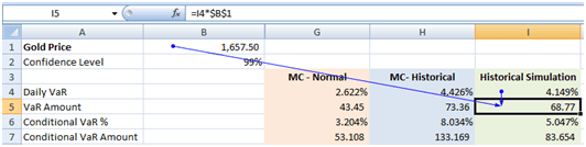
Once we calculate the daily VaR metric, the calculation of CVaR follows the same process for all three VaR approaches. As an example, we use the daily VaR from the Historical Simulation approach as an input in our CVaR worksheet. After we review the CVaR methodology we will present the results from all three methods.
To determine the expectation of loss given it exceeds the VaR level first calculate the loss incurred at the VaR level. Consider the following instance: Current Gold price is 1,657.50 and the daily VaR % using the Historical simulation approach is 4.149%. The loss at the VaR level or the price shock at the VaR level is 68.77.
Next, we determine the loss amounts. For each of the 364 returns, we calculate the price shocks in monetary terms. In the losses column, we will only consider the negative price shocks (i.e. price declines). For positive price shocks, we will consider a loss of zero.
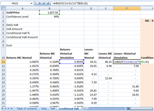
What is the conditional expectation of loss if the loss amount exceeds 68.77?
Conditional Value at Risk – Calculation methodology review
The methodology followed here is the same as that used for determining the conditional expectation or expected value of a roll of a fair die given that the value rolled is greater than a certain number.
First, let us consider the unconditional expectation of a six sided fair die. It is equal to the sum product of the value on the face of the die that turns up when rolled times the probability of that occurrence. For a fair die, as there are six possible occurrences, the probability of any value on a roll is 1/6. The unconditional expectation is then equal to 1*1/6 + 2*1/6 + 3*1/6 + 4*1/6 + 5*1/6 + 6*1/6 =21/6 =3.5
The conditional expectation is equal to the sum product of the value on face the die that turns up given that it is greater than a certain number times the probability of its occurrence. Supposing that it is given that the value rolled is greater than 3. There are three occurrences that meet this condition (4,5,6), each having an equal probability of occurrence, i.e. 1/3. The conditional expectation works out to 4*1/3 + 5*1/3 + 6*1/3 = 5
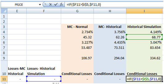
In a similar manner, once we determine the loss amounts for each data point, we factor in the condition that the loss amount exceeds 68.77, i.e. the VaR loss amount. This is factored in the worksheet as follows. We will only take losses that exceed 68.77 in the calculation, losses that are less than this amount are ignored. We may do this in one of two ways.
Conditional Loss Amount
Calculate a separate column that takes the loss amount as is if it exceeds 68.77 or replaces it with zero if it doesn’t.
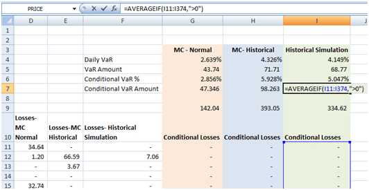
Conditional VaR Amount
We then apply the AVERAGEIF function to the array of these conditional losses so that we consider only those instances where the loss exceeds zero. Note that as we consider each return as a separate observation the probability of occurrence is 1/number of occurrences where the conditional loss is greater than zero. The conditional VaR amount or Expected Shortfall works out to 83.65 for a confidence level of 99%.
We may obtain the same result by directly applying the AVERAGEIF function to the array of unconditional losses and resetting the criteria from greater than zero to greater than the VaR Amount, i.e. =AVERAGEIF(F11:F374,CONCATENATE(“>”,I5)).
Conditional VaR %
The Conditional VaR % is then equal to the Conditional VaR Amount/ Current Value of the position = 83.65/1657.50 =5.047%. Determine CVaR% directly from the array of returns by applying the AVERAGEIF function to the array of returns and setting the criteria to the Daily VaR (%), specifically CVaR%=-AVERAGEIF(array of returns, CONCATENATE(“<“,-Daily VaR%).
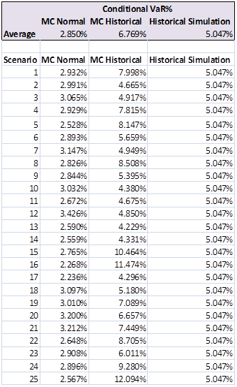
How do the results from the Monte Carlo simulation using the Historical returns approach compare with those obtained using the historical simulation method and the original MC-Normal approach? The average CVaR%s over 25 simulation runs are below:
Also, see Unexpected Loss (UL) and The Economic Capital Case Study if you are interested in extending the shortfall model for Economic Capital applications.